
Mathematics · Glossary

What is compact metric space?

Definition 4.15 University Mathematics — Year 2 · Chapter 4 — Topology of Metric Spaces

A metric space XX is compact when every sequence in XX has a subsequence converging in XX (the Bolzano–Weierstrass property). A subset is compact when it is so with the induced distance.
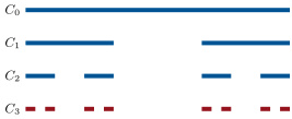
The first stages of the Cantor set (): each level deletes the open middle third of every segment. The intersection C = _n C_n is compact, has empty interior and length zero, yet is equipotent to ℝ — and it returns as a fixed point of a contraction on sets in this chapter’s weekend problem (question 22).
The first stages of the Cantor set (Exercise 4.8): each level deletes the open middle third of every segment. The intersection C=nCnC = \bigcap_n C_n is compact, has empty interior and length zero, yet is equipotent to R\R — and it returns as a fixed point of a contraction on sets in this chapter’s weekend problem (question 22).

Examples

Example 4.17 (Heine’s theorem, with and without compactness)

On [0,1]\intcc{0}{1}, the function xx2x \mapsto x^2 is uniformly continuous — Heine says so with no computation, but the direct estimate is instructive:

x2y2=x+yxy2xy,\abs{x^2 - y^2} = \abs{x + y}\,\abs{x - y} \leq 2\abs{x - y},

so δ=ε/2\delta = \varepsilon/2 works for every point at once. On R\R the same function is not uniformly continuous: with xn=nx_n = n and yn=n+1ny_n = n + \frac1n, the gap xnyn=1n0\abs{x_n - y_n} = \frac1n \to 0 while xn2yn2=2+1n22\abs{x_n^2 - y_n^2} = 2 + \frac1{n^2} \geq 2: no single δ\delta serves ε=1\varepsilon = 1. The mechanism is visible: the local Lipschitz constant x+y\abs{x + y} is bounded on a compact and unbounded on R\R — Heine’s theorem is exactly the statement that compactness caps such local constants uniformly.

Example 4.19 (Distances between sets: compactness earns its keep)

Let KK be compact, FF closed, KF=K \cap F = \emptyset in a metric space. Then

d(K,F)=inf{d(x,y):xK, yF}>0:d(K, F) = \inf\,\{d(x, y) : x \in K,\ y \in F\} > 0 :

the function xd(x,F)x \mapsto d(x, F) is continuous (Exercise 4.11) and positive on KK (d(x,F)=0d(x, F) = 0 would put xF=Fx \in \overline F = F), so it attains a positive minimum on the compact KK (Theorem 4.16 (3)). Compactness is not decorative: for two closed sets the infimum can vanish without being attained — in R2\R^2, the hyperbola F1={xy=1}F_1 = \{xy = 1\} and the axis F2={y=0}F_2 = \{y = 0\} are disjoint closed sets with d(F1,F2)=0d(F_1, F_2) = 0 (the points (n,1n)(n, \frac1n) approach the axis). Escape to infinity is exactly what compactness forbids.

Example 4.21 (An ε\varepsilon-net, counted)

Total boundedness (from the proof of Theorem 4.20) is very concrete on [0,1]\intcc{0}{1}: for ε>0\varepsilon > 0, the 12ε\lceil \frac{1}{2\varepsilon}\rceil balls centered at ε,3ε,5ε,\varepsilon, 3\varepsilon, 5\varepsilon, \dots of radius ε\varepsilon cover it — about 12ε\frac1{2\varepsilon} balls, and no cover can do with fewer than 12ε\frac{1}{2\varepsilon} of them (each ball covers length at most 2ε2\varepsilon). In [0,1]2\intcc01^2 the count squares to order ε2\varepsilon^{-2}: covering numbers grow like εd\varepsilon^{-d} in dimension dd — a quantitative face of compactness, and the reason the infinite-dimensional unit balls of Chapter 5 (where no finite 13\frac13-net exists at all) cannot be compact.

Read in context →