University Mathematics — Year 2 · Bachelor Year 2

4Topology of Metric Spaces

The topology of the real line (Year 1 volume) generalizes, almost without changing a word, to any set equipped with a distance. The gain is enormous: sequences of functions, matrices, curves — all become points of metric spaces, and the three pillars proved here — completeness with the Banach fixed point theorem, compactness, connectedness — apply to them uniformly. This chapter is the backbone of the whole analysis half of the book.

4.1 Metric spaces

Definition 4.1

A metric space is a set $X$ with a map $d \colon X \times X \to \R_+$ such that, for all $x, y, z$ :

d(x,y) = 0 \iff x = y, \qquad d(x,y) = d(y,x), \qquad d(x,z) \leq d(x,y) + d(y,z).

Balls: $B(a, r) = \{x : d(a,x) < r\}$ (open), $\overline B(a,r) = \{x : d(a,x) \leq r\}$ (closed). A subset $A \subseteq X$ becomes a metric space with the induced distance.

Example 4.2

$\R$ with $\abs{x - y}$ ; $\R^n$ with any of

d_1(x,y) = \sum_i \abs{x_i - y_i}, \quad d_2(x,y) = \Bigl(\sum_i (x_i - y_i)^2\Bigr)^{1/2}, \quad d_\infty(x,y) = \max_i \abs{x_i - y_i};

the set $C(\intcc{a}{b})$ of continuous functions with the sup distance $d_\infty(f, g) = \sup_{\intcc{a}{b}} \abs{f - g}$ (finite: $f - g$ is bounded); any set with the discrete distance ( $d(x,y) = 1$ for $x \neq y$ ). Distances coming from norms are the subject of Chapter 5.

Definition 4.3 (Topology of a metric space)

$U \subseteq X$ is open when every point of $U$ is the center of a ball contained in $U$ ; $F$ is closed when its complement is open. Neighborhoods, interior, closure, density, boundary are defined exactly as on the real line (Year 1 volume), with balls replacing intervals, and the statements proved there — unions/intersections of open sets, characterizations of interior and closure, closure as smallest closed superset — carry over with the same proofs. Open balls are open, closed balls are closed (triangle inequality).

Example 4.4 (Interior, closure, boundary on one set)

In $\R$ , let $A = \intoc{0}{1} \cup \{2\}$ . Interior: $\intoo{0}{1}$ — around any $x \in \intoo01$ a small ball stays in $A$ ; around $1$ , every ball $\intoo{1-r}{1+r}$ leaks out of $A$ on the right, so $1$ is not interior; and the isolated $2$ is not interior either. Closure: $\intcc{0}{1} \cup \{2\}$ (the point $0$ is a limit of $A$ , nothing else is added). Boundary (closure minus interior): $\{0, 1, 2\}$ . Note the asymmetries worth remembering: an endpoint can belong to a set without being interior ( $1$ ), can be adherent without belonging ( $0$ ), and an isolated point is its own boundary ( $2$ ). The same bookkeeping runs verbatim in any metric space, with balls in place of intervals.

Definition 4.5 (Limits, continuity)

$x_n \to x$ in $X$ when $d(x_n, x) \to 0$ . A map $f \colon X \to Y$ between metric spaces is continuous at $a$ when

\forall \varepsilon > 0,\ \exists\delta > 0,\quad d_X(x, a) \leq \delta \implies d_Y\bigl(f(x), f(a)\bigr) \leq \varepsilon ;

equivalently (same proof as on $\R$ ), $f(x_n) \to f(a)$ for every sequence $x_n \to a$ . $f$ is Lipschitz with constant $k$ when $d_Y(f(x), f(y)) \leq k\, d_X(x, y)$ always — then uniformly continuous, hence continuous.

Theorem 4.6 (Global characterization of continuity)

$f \colon X \to Y$ is continuous (at every point) if and only if the preimage of every open set is open — iff the preimage of every closed set is closed.

Proof. ( $\Rightarrow$ ) Let $V \subseteq Y$ be open and $a \in f^{-1}(V)$ : some ball $B(f(a), \varepsilon) \subseteq V$ ; continuity at $a$ provides $\delta$ with $f(B(a, \delta)) \subseteq B(f(a), \varepsilon)$ , so $B(a, \delta) \subseteq f^{-1}(V)$ .

( $\Leftarrow$ ) Given $a$ and $\varepsilon$ : $f^{-1}\bigl(B(f(a), \varepsilon)\bigr)$ is open and contains $a$ , hence contains a ball $B(a, \delta)$ : that is the definition of continuity at $a$ . Closed sets: complements (Proposition 1.1). ∎

4.2 Complete spaces

Definition 4.7

A sequence $(x_n)$ is Cauchy when $\sup_{p, q \geq N} d(x_p, x_q) \to 0$ as $N \to \infty$ . A metric space is complete when every Cauchy sequence converges. Convergent $\Rightarrow$ Cauchy always; closed subsets of complete spaces are complete, and complete subsets of any space are closed (same proofs as on $\R$ : Year 1 volume).

Example 4.8 (Cauchy without a limit)

In $X = \Q$ with the usual distance, the decimal truncations of $\sqrt2$ ,

x_0 = 1,\quad x_1 = 1.4,\quad x_2 = 1.41,\quad x_3 = 1.414, \quad\dots

satisfy $\abs{x_p - x_q} \leq 10^{-\min(p,q)}$ : Cauchy in $\Q$ . A limit in $\Q$ would also be the limit in $\R$ , namely $\sqrt2 \notin \Q$ : no limit exists in $X$ . Incompleteness is the presence of such “phantom limits”; completeness of $\R$ was engineered in the Year 1 volume precisely to give every Cauchy sequence a home.

Theorem 4.9

$\R^n$ (any of the three distances of Example 4.2) and $\bigl(C(\intcc{a}{b}), d_\infty\bigr)$ are complete.

Proof. $\R^n$ : a Cauchy sequence is Cauchy in each coordinate (each $\abs{x_i - y_i} \leq d(x,y)$ for all three distances), so each coordinate converges (completeness of $\R$ , Year 1 volume), and coordinatewise convergence implies convergence for $d_\infty$ (finitely many coordinates), hence for all three (the three distances dominate each other within constant factors: $d_\infty \leq d_2 \leq d_1 \leq n\,d_\infty$ ).

$C(\intcc{a}{b})$ : let $(f_n)$ be $d_\infty$ -Cauchy. For each $x$ , $(f_n(x))$ is Cauchy in $\R$ ( $\abs{f_p(x) - f_q(x)} \leq d_\infty(f_p, f_q)$ ): converges to some $f(x)$ . Passing to the limit in $\abs{f_p(x) - f_q(x)} \leq \varepsilon$ (valid for $p, q \geq N_\varepsilon$ , all $x$ ) as $q \to \infty$ : $\abs{f_p(x) - f(x)} \leq \varepsilon$ for all $x$ , i.e. $d_\infty(f_p, f) \leq \varepsilon$ : uniform convergence. The limit is continuous: given $\varepsilon$ , pick $p$ with $\sup\abs{f_p - f} \leq \varepsilon$ , then use continuity of $f_p$ at $a$ and the three-term split

\abs{f(x) - f(a)} \leq \abs{f(x) - f_p(x)} + \abs{f_p(x) - f_p(a)} + \abs{f_p(a) - f(a)} \leq 3\varepsilon

for $x$ close to $a$ . (This “ $3\varepsilon$ argument” returns as the uniform-limit theorem of Chapter 10.) ∎

Example 4.10 (Open and closed sets recognized by continuity)

The global characterization (Theorem 4.6) is the everyday tool for topological bookkeeping. In $\R^2$ : the set $\{(x, y) : x^2 + y^2 < 1,\ y > x^3\}$ is open — it is $g^{-1}(\intoo{-\infty}{1}) \cap h^{-1}(\intoo{0}{+\infty})$ for the continuous $g(x,y) = x^2 + y^2$ and $h(x, y) = y - x^3$ , an intersection of two open preimages. In $\bigl(C(\intcc01), d_\infty\bigr)$ : the set of functions with $f(0) = f(1)$ and $\int_0^1 f = 0$ is closed — the preimage of $\{(0,0)\}$ under the continuous map $f \mapsto \bigl(f(0) - f(1),\ \int_0^1 f\bigr)$ into $\R^2$ (each coordinate is $1$ -Lipschitz, as in Exercise 4.3). The method never draws a picture: exhibit a continuous map, read the set as a preimage, quote the theorem.

Example 4.11 (A closed set defined by infinitely many conditions)

In $\bigl(C(\intcc01), d_\infty\bigr)$ , the set

L = \{f : \abs{f(x) - f(y)} \leq \abs{x - y} \ \text{for all } x, y\}

of $1$ -Lipschitz functions is closed, although it is cut out by uncountably many conditions: for each fixed pair $(x, y)$ , the map $f \mapsto \abs{f(x) - f(y)} - \abs{x - y}$ is continuous (evaluations are $1$ -Lipschitz), so each single condition defines a closed set, and $L$ is the intersection of this family — an arbitrary intersection of closed sets is closed. The same template certifies closedness for monotone functions, convex functions, functions bounded by a fixed $g$ : uniform limits inherit every property expressible as a family of closed pointwise constraints. What uniform limits do not automatically inherit — differentiability, for one — is exactly what Chapter 10 must labour for.

Theorem 4.12 (Banach fixed point theorem)

Let $X$ be a nonempty complete metric space and $f \colon X \to X$ a contraction: Lipschitz with constant $k < 1$ . Then $f$ has a unique fixed point $\ell$ , and every orbit $x_{n+1} = f(x_n)$ converges to $\ell$ , with

d(x_n, \ell) \leq \frac{k^n}{1 - k}\, d(x_1, x_0) .

Proof. Uniqueness: two fixed points are at distance $\leq k$ times itself. Existence: $d(x_{n+1}, x_n) \leq k^n d(x_1, x_0)$ by induction, so for $q > p$ ,

d(x_q, x_p) \leq \sum_{j=p}^{q-1} d(x_{j+1}, x_j) \leq d(x_1, x_0) \sum_{j \geq p} k^j = \frac{k^p}{1-k}\, d(x_1, x_0) \xrightarrow[p\to\infty]{} 0 :

Cauchy, hence convergent to some $\ell$ ; continuity of $f$ passes $x_{n+1} = f(x_n)$ to the limit: $\ell = f(\ell)$ . The error bound is the displayed estimate with $q \to \infty$ . ∎

Example 4.13 (An integral equation)

On $X = C(\intcc{0}{1})$ (complete, Theorem 4.9), consider $T(f)(x) = 1 + \frac12 \int_0^x f(t)\,\dd t$ . For $f, g \in X$ :

\abs{T(f)(x) - T(g)(x)} \leq \frac12 \int_0^x \abs{f - g} \leq \frac12\, d_\infty(f, g),

so $T$ is a $\frac12$ -contraction: it has a unique continuous fixed point — the solution of $f' = \frac f2$ , $f(0) = 1$ , namely $\eu^{x/2}$ . This scheme, industrialized, becomes the Cauchy–Lipschitz theorem of Chapter 16.

Example 4.14 (A numerical fixed point: $x = \cos x$ )

On the complete $X = \intcc{0}{1}$ , the map $f = \cos$ sends $X$ into $\intcc{\cos 1}{1} \subseteq X$ and is a contraction: by the mean value inequality,

\abs{\cos x - \cos y} \leq \bigl(\sup_{\intcc01}\abs{\sin}\bigr) \abs{x - y} = (\sin 1)\abs{x - y}, \qquad \sin 1 \approx 0.841 < 1 .

Banach: a unique solution of $x = \cos x$ in $\intcc01$ (hence in $\R$ : any real fixed point lies in $\intcc{-1}{1}$ , then in $\intcc{\cos 1}{1}$ after one application), and the iteration $x_{n+1} = \cos x_n$ converges to it from any start: $x_\infty \approx 0.739085$ , the famous number obtained by hammering the cosine key of a calculator. The error bound predicts $(\sin1)^n/(1 - \sin1)$ decay — about one digit per $13$ presses; the a posteriori bound of this chapter’s weekend problem (question 14) certifies each step on the fly.

4.3 Compactness

Definition 4.15

A metric space $X$ is compact when every sequence in $X$ has a subsequence converging in $X$ (the Bolzano–Weierstrass property). A subset is compact when it is so with the induced distance.

Theorem 4.16 (First properties)

A compact subset is closed and bounded; a closed subset of a compact space is compact.
In $\R^n$ , the converse holds: compact $\iff$ closed and bounded.
A continuous image of a compact space is compact; a continuous real function on a nonempty compact space is bounded and attains its bounds.
(Heine) A continuous map on a compact space is uniformly continuous.
Products: if $X, Y$ are compact, so is $X \times Y$ (with $d\bigl((x,y),(x',y')\bigr) = d(x,x') + d(y,y')$ ).

Proof. (1) Same arguments as on the line (Year 1 volume): an escaping-to- infinity or converging-outside sequence has no subsequence converging inside; for the second claim, extract in the ambient compact and use closedness.

(2) Bounded sequences in $\R^n$ have componentwise convergent subsequences: extract on the first coordinate (Bolzano–Weierstrass on $\R$ ), then, from that subsequence, on the second, and so on ( $n$ successive extractions); closedness keeps the limit inside.

(3) Given $(f(x_n))$ , extract $x_{\varphi(n)} \to x \in X$ ; continuity gives $f(x_{\varphi(n)}) \to f(x) \in f(X)$ . Real case: compactness of $f(X) \subseteq \R$ makes it closed and bounded, and $\sup f(X) \in f(X)$ (the sup of a set is adherent to it, and $f(X)$ is closed).

(4) The Year 1 proof transfers verbatim; here it is, in metric dress. Suppose $f \colon X \to Y$ continuous on the compact $X$ but not uniformly continuous: some $\varepsilon > 0$ admits, for every $n$ , points with

d_X(x_n, y_n) \leq \frac{1}{n+1} \qquad\text{and}\qquad d_Y\bigl(f(x_n), f(y_n)\bigr) > \varepsilon .

Extract $x_{\varphi(n)} \to a \in X$ ; then $y_{\varphi(n)} \to a$ too (the mutual distances tend to $0$ ). Continuity at $a$ sends both image sequences to $f(a)$ , so $d_Y\bigl(f(x_{\varphi(n)}), f(y_{\varphi(n)})\bigr) \to 0$ — contradicting the uniform gap $> \varepsilon$ . Compactness supplied exactly one thing: the cluster point $a$ at which to apply plain continuity.

(5) Extract on the $X$ -coordinates, then again on the $Y$ -coordinates. ∎

Example 4.17 (Heine’s theorem, with and without compactness)

On $\intcc{0}{1}$ , the function $x \mapsto x^2$ is uniformly continuous — Heine says so with no computation, but the direct estimate is instructive:

\abs{x^2 - y^2} = \abs{x + y}\,\abs{x - y} \leq 2\abs{x - y},

so $\delta = \varepsilon/2$ works for every point at once. On $\R$ the same function is not uniformly continuous: with $x_n = n$ and $y_n = n + \frac1n$ , the gap $\abs{x_n - y_n} = \frac1n \to 0$ while $\abs{x_n^2 - y_n^2} = 2 + \frac1{n^2} \geq 2$ : no single $\delta$ serves $\varepsilon = 1$ . The mechanism is visible: the local Lipschitz constant $\abs{x + y}$ is bounded on a compact and unbounded on $\R$ — Heine’s theorem is exactly the statement that compactness caps such local constants uniformly.

Method 4.18 (Proving that a set is compact)

Three routes, in order of frequency. (1) Ambient recognition: in $\R^n$ (or any finite-dimensional normed space, Chapter 5), verify closed — typically as a preimage, Example 4.10 — and bounded. (2) Inheritance: a closed subset of a known compact space is compact; a finite union or a product of compacts is compact; a continuous image of a compact is compact. (3) Bare hands: extract a convergent subsequence from an arbitrary sequence — usually by successive extractions coordinate by coordinate. To prove non-compactness, one witness suffices: a sequence with no convergent subsequence, most often points at mutual distance $\geq \varepsilon$ .

Example 4.19 (Distances between sets: compactness earns its keep)

Let $K$ be compact, $F$ closed, $K \cap F = \emptyset$ in a metric space. Then

d(K, F) = \inf\,\{d(x, y) : x \in K,\ y \in F\} > 0 :

the function $x \mapsto d(x, F)$ is continuous (Exercise 4.11) and positive on $K$ ( $d(x, F) = 0$ would put $x \in \overline F = F$ ), so it attains a positive minimum on the compact $K$ (Theorem 4.16 (3)). Compactness is not decorative: for two closed sets the infimum can vanish without being attained — in $\R^2$ , the hyperbola $F_1 = \{xy = 1\}$ and the axis $F_2 = \{y = 0\}$ are disjoint closed sets with $d(F_1, F_2) = 0$ (the points $(n, \frac1n)$ approach the axis). Escape to infinity is exactly what compactness forbids.

Theorem 4.20 (Borel–Lebesgue)

A metric space $X$ is compact if and only if every cover of $X$ by open sets has a finite subcover.

Proof. ( $\Leftarrow$ ) Suppose $(x_n)$ has no convergent subsequence. We claim every $x \in X$ has a ball $B(x, r_x)$ containing $x_n$ for only finitely many indices $n$ : otherwise, every ball $B(x, \frac1{k+1})$ would contain infinitely many terms, and choosing indices

\varphi(0) < \varphi(1) < \varphi(2) < \cdots \quad\text{with}\quad x_{\varphi(k)} \in B\Bigl(x, \frac{1}{k+1}\Bigr)

(possible at each step precisely because infinitely many candidates remain) would build a subsequence converging to $x$ . The balls $B(x, r_x)$ cover $X$ ; if finitely many of them covered $X$ , the index set $\N$ would be a finite union of finite sets: absurd.

( $\Rightarrow$ ) Two steps. Lebesgue number: for an open cover $(U_i)$ of a compact $X$ , there is $\rho > 0$ such that every ball of radius $\rho$ lies in some $U_i$ . Otherwise, for each $n$ pick $x_n$ with $B(x_n, \frac{1}{n+1})$ in no $U_i$ ; extract $x_{\varphi(n)} \to x \in U_{i_0} \supseteq B(x, r)$ ; for large $n$ , $B(x_{\varphi(n)}, \frac{1}{\varphi(n)+1}) \subseteq B(x, r) \subseteq U_{i_0}$ : contradiction. Total boundedness: for every $\rho > 0$ , finitely many balls of radius $\rho$ cover $X$ . Otherwise pick inductively $x_{n+1}$ outside $B(x_0, \rho) \cup \dots \cup B(x_n, \rho)$ : the sequence has pairwise distances $\geq \rho$ , so no Cauchy — hence no convergent — subsequence: contradiction. Combining: cover $X$ by finitely many balls of radius $\rho$ (the Lebesgue number), each inside some $U_i$ : a finite subcover. ∎

Example 4.21 (An $\varepsilon$ -net, counted)

Total boundedness (from the proof of Theorem 4.20) is very concrete on $\intcc{0}{1}$ : for $\varepsilon > 0$ , the $\lceil \frac{1}{2\varepsilon}\rceil$ balls centered at $\varepsilon, 3\varepsilon, 5\varepsilon, \dots$ of radius $\varepsilon$ cover it — about $\frac1{2\varepsilon}$ balls, and no cover can do with fewer than $\frac{1}{2\varepsilon}$ of them (each ball covers length at most $2\varepsilon$ ). In $\intcc01^2$ the count squares to order $\varepsilon^{-2}$ : covering numbers grow like $\varepsilon^{-d}$ in dimension $d$ — a quantitative face of compactness, and the reason the infinite-dimensional unit balls of Chapter 5 (where no finite $\frac13$ -net exists at all) cannot be compact.

Example 4.22 (Reading compactness on covers)

The half-open interval $\intoc{0}{1}$ is covered by the open sets $U_n = \intoo{\frac1n}{2}$ , $n \geq 1$ ; any finite subfamily has a largest index $N$ and misses $\intoc{0}{\frac1N}$ : no finite subcover, so $\intoc{0}{1}$ is not compact — which the sequential definition sees through $x_n = \frac1n$ , whose limit $0$ escapes. On the other hand, adding the single point $0$ repairs both diagnoses at once: on $\intcc{0}{1}$ every such cover must contain a set containing $0$ , which swallows a whole initial segment, and finitely many sets finish the rest. The two languages of Theorem 4.20 always fail or succeed together — covers detect escape exactly where sequences do.

Remark 4.23 (Perspectives within this volume)

This chapter is the volume’s load-bearing wall; watch where each pillar carries weight. Completeness: the Cauchy criterion becomes the convergence test for series in Banach spaces (Chapter 7), uniform convergence in Chapter 10 is exactly convergence in the complete $\bigl(C, d_\infty\bigr)$ , and Cauchy–Lipschitz (Chapter 16) is the Banach fixed point theorem wearing an integral equation. Compactness: it proves the equivalence of norms (Chapter 5), the attainment of extrema for the optimization of Chapter 15, and the existence of best approximations (Chapter 5’s weekend problem). Connectedness: it globalizes local statements — uniqueness of solutions of differential equations, the intermediate value theorem on curves (Chapter 18), and the two components of $GL_n(\R)$ that orientation theory (Chapter 20) will keep apart.

Remark 4.24 (Common pitfalls)

(i) “Closed and bounded implies compact” is a theorem about $\R^n$ , not about metric spaces: an infinite set with the discrete metric is closed and bounded in itself yet not compact (Exercise 4.4), and the closed unit ball of $C(\intcc01)$ fails too (Chapter 5). (ii) Completeness is a property of the distance, not of the topology: $\R$ with $d(x,y) = \abs{\arctan x - \arctan y}$ has the usual convergent sequences but is incomplete (Exercise 4.1). (iii) A continuous bijection need not be a homeomorphism — the circle parametrization of Exercise 4.7; compactness of the source repairs it. (iv) Banach’s theorem needs $k < 1$ uniformly: the condition $d(f(x), f(y)) < d(x,y)$ alone guarantees nothing on a non-compact space (Exercise 4.5). (v) Connected does not imply path-connected in general — but for the open subsets of normed spaces met in this book, the two agree (Chapter 5).

Remark 4.25 (Where this chapter is used)

Everywhere in the analysis half. Completeness of $C(\intcc{a}{b})$ powers the convergence theorems of Chapter 10 and the Cauchy–Lipschitz theory of Chapter 16 (this chapter’s weekend problem proves the local Picard–Lindelöf theorem already); compactness gives the equivalence of norms in finite dimension (Chapter 5) and the existence of extrema in Chapter 15; connectedness underlies the intermediate value arguments of Chapter 8 and the uniqueness globalization for differential equations. In the Year 3 volume, compactness in function spaces (the Arzelà–Ascoli theorem) and the Baire category theorem (Exercise 4.12 here) become tools of daily use.

The first stages of the Cantor set (): each level deletes the open middle third of every segment. The intersection C = _n C_n is compact, has empty interior and length zero, yet is equipotent to ℝ — and it returns as a fixed point of a contraction on sets in this chapter’s weekend problem (question 22). — The first stages of the Cantor set (Exercise 4.8): each level deletes the open middle third of every segment. The intersection $C = \bigcap_n C_n$ is compact, has empty interior and length zero, yet is equipotent to $\R$ — and it returns as a *fixed point* of a contraction on sets in this chapter’s weekend problem (question 22).

4.4 Connectedness

Definition 4.26

$X$ is connected when it admits no partition into two nonempty open subsets — equivalently, when its only subsets both open and closed are $\emptyset$ and $X$ . $X$ is path-connected when any two points are joined by a continuous map $\gamma \colon \intcc{0}{1} \to X$ .

Theorem 4.27

The connected subsets of $\R$ are exactly the intervals.
A continuous image of a connected space is connected — whence the general intermediate value theorem: a continuous real function on a connected space takes every value between any two of its values.
Path-connected $\Rightarrow$ connected. (The converse fails in general; it holds for open subsets of normed spaces, Chapter 5.)

Proof. (1) A non-interval $A$ misses some $z$ between two of its points: $A = (A \cap \intoo{-\infty}{z}) \cup (A \cap \intoo{z}{+\infty})$ splits it into two nonempty open (in $A$ ) pieces. Conversely, let $I$ be an interval and $I = U \cup V$ a partition into nonempty relatively open sets; pick $a \in U$ , $b \in V$ , say $a < b$ , and set $s = \sup\,(U \cap \intcc{a}{b})$ , a point of $\intcc{a}{b} \subseteq I$ . If $s \in U$ : then $s \neq b$ , and relative openness of $U$ puts a whole interval around $s$ (intersected with $I$ ) inside $U$ — so points of $U \cap \intcc{a}{b}$ exceed $s$ , contradicting the supremum. If $s \in V$ : relative openness of $V$ puts an interval $\intoo{s - r}{s + r} \cap I$ inside $V$ ; but the supremum is adherent to $U \cap \intcc{a}{b}$ , which must meet that interval — contradiction with $U \cap V = \emptyset$ . (This is the Year 1 clopen argument for $\R$ , run inside $I$ .)

(2) If $f(X) = U' \cup V'$ splits into nonempty relatively open sets, then $X = f^{-1}(U') \cup f^{-1}(V')$ splits $X$ (Theorem 4.6). IVT: $f(X) \subseteq \R$ is connected, hence an interval by (1).

(3) Suppose $X = U \cup V$ , both nonempty open, and join $a \in U$ to $b \in V$ by a path $\gamma$ : then $\gamma^{-1}(U), \gamma^{-1}(V)$ split $\intcc{0}{1}$ , contradicting (1). ∎

Example 4.28

$GL_n(\R)$ is not connected: $\det$ is continuous (a polynomial in the entries) onto $\R^*$ , which is not connected; the preimages of $\R_+^*$ and $\R_-^*$ split $GL_n(\R)$ . (Each piece is in fact path-connected — a pleasant exercise beyond our needs.) By contrast $GL_n(\C)$ is path-connected: Exercise 4.10.

Example 4.29 (A fixed point from connectedness alone)

Every continuous $f \colon \intcc01 \to \intcc01$ has a fixed point — no contraction hypothesis, no iteration. Consider $g(x) = f(x) - x$ , continuous on the connected $\intcc01$ :

g(0) = f(0) \geq 0, \qquad g(1) = f(1) - 1 \leq 0 ,

and the intermediate value theorem (Theorem 4.27 (2)) delivers a zero of $g$ , i.e. a fixed point of $f$ . Contrast with Banach (Theorem 4.12): here existence is topological and free, but uniqueness and the algorithm are lost — $f = \mathrm{id}$ has every point fixed, and iteration of a non-contracting $f$ may cycle forever. The two fixed point theorems of this chapter answer different questions with different currencies.

Example 4.30 ( $\R$ and $\R^2$ are not homeomorphic)

Connectedness is a topological fingerprint. Suppose $h \colon \R^2 \to \R$ were a homeomorphism (a continuous bijection with continuous inverse). Remove one point $a \in \R^2$ : the restriction $h \colon \R^2\setminus\{a\} \to \R\setminus\{h(a)\}$ is still a homeomorphism. But $\R^2$ minus a point is path-connected — join any two points by a segment, detouring along a second segment through an auxiliary point if $a$ blocks the direct one — hence connected (Theorem 4.27 (3)); while $\R$ minus a point splits into two nonempty open half-lines: not connected. Connectedness is preserved by continuous maps: contradiction. The plane and the line are genuinely different as topological spaces — a fact that cardinality alone (Exercise 1.3-style bijections do exist!) is too coarse to see.

4.5 Exercises

Exercise 4.1 ★

On $\R$ , check that $\delta(x, y) = \min(1, \abs{x - y})$ and $d(x,y) = \abs{\arctan x - \arctan y}$ are distances. Which sequences converge for each? Is $(\R, d)$ complete?

Solution

Solution of Exercise 4.1.

$\delta$ : symmetry and separation are clear; triangle inequality: $\min(1, u + v) \leq \min(1,u) + \min(1,v)$ for $u, v \geq 0$ (if either min is $1$ , the right side is $\geq 1$ ; else it is $u + v$ ). $d$ : it is the pullback of $\abs{\cdot}$ by the injective $\arctan$ : the three axioms transfer.

Convergence: for $\delta$ , $\delta(x_n, x) \to 0 \iff \abs{x_n - x} \to 0$ (for small values the two distances agree): same convergent sequences as usual. For $d$ : $d(x_n, x) \to 0 \iff \arctan x_n \to \arctan x \iff x_n \to x$ (continuity and strict monotonicity of $\arctan$ and of its inverse on the relevant ranges): again the usual convergence.

$(\R, d)$ is not complete: $x_n = n$ satisfies $d(x_p, x_q) = \abs{\arctan p - \arctan q} \to 0$ (both tend to $\frac\pi2$ ): Cauchy; but $(x_n)$ does not converge for $d$ (its $d$ -limit would be an ordinary limit). Completeness is a property of the distance, not just of the convergent sequences.

Exercise 4.2 ★

In a metric space, prove that a convergent sequence is Cauchy and bounded, and that a Cauchy sequence with a convergent subsequence converges. Deduce again that compact metric spaces are complete.

Solution

Solution of Exercise 4.2.

Convergent $\Rightarrow$ Cauchy: $d(x_p, x_q) \leq d(x_p, \ell) + d(\ell, x_q)$ . Bounded: beyond $N$ , $d(x_n, \ell) \leq 1$ ; the finitely many first terms are within some radius too.

Cauchy $+$ convergent subsequence $x_{\varphi(n)} \to \ell$ : given $\varepsilon$ , for large $n$ , $d(x_n, \ell) \leq d(x_n, x_{\varphi(n)}) + d(x_{\varphi(n)}, \ell) \leq 2\varepsilon$ (the first term by Cauchy, since $\varphi(n) \geq n$ ).

Compact $\Rightarrow$ complete: a Cauchy sequence has a convergent subsequence (compactness), hence converges.

Exercise 4.3 ★

In $\bigl(C(\intcc{0}{1}), d_\infty\bigr)$ , compute the distance between $f(x) = x$ and $g(x) = x^2$ ; describe the closed ball $\overline B(0, 1)$ ; and prove that the set $\{f : f(0) = 0\}$ is closed while $\{f : f(0) > 0\}$ is open.

Solution

Solution of Exercise 4.3.

$d_\infty(f, g) = \sup_{\intcc{0}{1}} \abs{x - x^2} = \frac14$ (maximum of $x - x^2$ at $x = \frac12$ ).

$\overline B(0, 1) = \{f : \sup\abs f \leq 1\}$ : the continuous functions with values in $\intcc{-1}{1}$ .

$\{f : f(0) = 0\}$ is the preimage of $\{0\}$ under the evaluation $f \mapsto f(0)$ , which is $1$ -Lipschitz ( $\abs{f(0) - g(0)} \leq d_\infty(f,g)$ ), hence continuous: the set is closed (Theorem 4.6). Likewise $\{f : f(0) > 0\}$ is the preimage of the open $\intoo{0}{+\infty}$ : open.

Exercise 4.4 ★★

Prove that the discrete metric space $X$ (any set) is complete, and that it is compact if and only if $X$ is finite. Which subsets are connected?

Solution

Solution of Exercise 4.4.

Complete: a Cauchy sequence with $\varepsilon = \frac12$ is eventually constant, hence convergent.

Compact iff finite: if $X$ is finite, any sequence takes some value infinitely often (constant subsequence). If $X$ is infinite, a sequence of pairwise distinct points has all mutual distances $1$ : no Cauchy subsequence, so no convergent one.

Connected subsets: the singletons (and $\emptyset$ ). Any $A$ with two points $x \neq y$ splits as $\{x\} \cup (A \setminus\{x\})$ , both open in $A$ (every subset of a discrete space is open — balls of radius $\frac12$ are singletons).

Exercise 4.5 ★★

Let $X$ be compact and $f \colon X \to X$ with

d\bigl(f(x), f(y)\bigr) < d(x, y) \quad \text{for all } x \neq y .

Prove that $f$ has a unique fixed point (minimize $x \mapsto d(x, f(x))$ ), and give an example on $X = \intco{1}{+\infty}$ (not compact) with no fixed point.

Solution

Solution of Exercise 4.5.

The function $g(x) = d(x, f(x))$ is continuous on the compact $X$ ( $\abs{g(x) - g(y)} \leq 2d(x,y)$ by two triangle inequalities), so it attains its minimum at some $a$ (Theorem 4.16). If $f(a) \neq a$ :

g\bigl(f(a)\bigr) = d\bigl(f(a), f(f(a))\bigr) < d(a, f(a)) = g(a),

contradicting minimality. So $f(a) = a$ ; uniqueness as usual (two fixed points $a \neq b$ give $d(a,b) = d(f(a), f(b)) < d(a,b)$ ).

Non-compact example: $f(x) = x + \frac1x$ on $\intco{1}{+\infty}$ : $\abs{f(x) - f(y)} = \abs{x - y}\,\abs{1 - \frac{1}{xy}} < \abs{x - y}$ for $x \neq y$ (as $xy > 1$ ), yet $f(x) > x$ everywhere.

Exercise 4.6 ★★

(Nested compacts) Let $(K_n)$ be a decreasing sequence of nonempty compact subsets of a metric space. Prove that $\bigcap_n K_n \neq \emptyset$ (pick $x_n \in K_n$ and extract). Show by example that nonempty nested closed sets in $\R$ can have empty intersection.

Solution

Solution of Exercise 4.6.

Pick $x_n \in K_n$ . All terms from rank $n$ on lie in $K_n$ ; in particular the whole sequence lies in the compact $K_0$ : extract $x_{\varphi(k)} \to \ell$ . For each fixed $n$ , the terms $x_{\varphi(k)}$ with $\varphi(k) \geq n$ lie in the closed $K_n$ , so the limit $\ell \in K_n$ . Hence $\ell \in \bigcap K_n$ .

Closed counterexample: $F_n = \intco{n}{+\infty}$ in $\R$ : nested, closed, nonempty, empty intersection.

Exercise 4.7 ★★

Let $K$ be compact and $f \colon K \to Y$ continuous and bijective. Prove that $f^{-1}$ is continuous (use closed sets: Theorem 4.6 and Theorem 4.16). Give a counterexample without compactness ( $\gamma(t) = (\cos t, \sin t)$ on $\intco{0}{2\pi}$ ).

Solution

Solution of Exercise 4.7.

Continuity of $f^{-1}$ means: images $f(F)$ of closed sets $F \subseteq K$ are closed (preimages under $f^{-1}$ are images under $f$ ). A closed $F$ in the compact $K$ is compact (Theorem 4.16 (1)); its continuous image $f(F)$ is compact, hence closed. So $f^{-1}$ is continuous: $f$ is a homeomorphism.

Counterexample: $\gamma(t) = (\cos t, \sin t)$ from $\intco{0}{2\pi}$ (not compact) onto the unit circle is a continuous bijection, but $\gamma^{-1}$ is discontinuous at $(1,0)$ : points on the circle just below the axis have parameters near $2\pi$ , not near $0$ .

Exercise 4.8 ★★

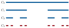
The Cantor set $C$ is obtained from $\intcc{0}{1}$ by repeatedly deleting open middle thirds. Prove that $C$ is compact, has empty interior, and is infinite — indeed equipotent to $\{0,1\}^{\N}$ (ternary expansions with digits $0,2$ ; Exercise 1.3).

Solution

Solution of Exercise 4.8.

$C = \bigcap_n C_n$ where each $C_n$ (union of $2^n$ closed intervals of length $3^{-n}$ ) is closed: $C$ is closed and bounded in $\R$ , hence compact (Theorem 4.16 (2)).

Empty interior: $C$ contains no interval of length $> 3^{-n}$ (it sits inside $C_n$ , whose components have that length), for every $n$ .

Cardinality: the points of $C$ are exactly the reals $\sum_{n\geq1} a_n 3^{-n}$ with digits $a_n \in \{0, 2\}$ (at each stage, the deleted middle third removes the digit $1$ ); the map $(a_n) \mapsto \sum a_n 3^{-n}$ is a bijection from $\{0,2\}^{\N^*}$ onto $C$ (injectivity as in Exercise 1.3). So $C$ is equipotent to $\{0,1\}^{\N}$ : uncountable, though of “length zero”.

Exercise 4.9 ★★★

Let $X$ be a compact metric space and $f \colon X \to X$ an isometry: $d(f(x), f(y)) = d(x, y)$ . Prove that $f$ is surjective. Hint: if $a \notin f(X)$ , then $\varepsilon = d(a, f(X)) > 0$ (why?); study the orbit $a, f(a), f^2(a), \dots$ and show its points are pairwise $\geq \varepsilon$ apart — contradiction with compactness.

Solution

Solution of Exercise 4.9.

Suppose $a \notin f(X)$ . The image $f(X)$ is compact (continuous image), hence closed; so

\varepsilon = d\bigl(a, f(X)\bigr) = \inf_{y \in f(X)} d(a, y) > 0

(the infimum of a continuous function on a compact set is attained; if it were $0$ , $a$ would be adherent to the closed $f(X)$ , hence in it).

Consider the orbit $x_n = f^n(a)$ ( $x_0 = a$ ). For $p < q$ :

d(x_p, x_q) = d\bigl(f^p(a), f^p(f^{q-p}(a))\bigr) = d\bigl(a, f^{q-p}(a)\bigr) \geq \varepsilon,

(isometry iterated $p$ times; and $f^{q-p}(a) \in f(X)$ since $q - p \geq 1$ ). A sequence with mutual distances $\geq \varepsilon$ has no convergent subsequence — contradicting compactness. Hence $f(X) = X$ .

Exercise 4.10 ★★★

Prove that $GL_n(\C)$ is path-connected. Hint: given $A, B$ invertible, consider $p(z) = \det\bigl((1 - z)A + zB\bigr)$ for $z \in \C$ : a polynomial in $z$ , not identically zero, so it has finitely many roots; join $0$ to $1$ in $\C$ by a path avoiding them.

Solution

Solution of Exercise 4.10.

Let $A, B \in GL_n(\C)$ and $p(z) = \det\bigl((1-z)A + zB\bigr)$ : a polynomial in $z$ (each entry is affine in $z$ ; the determinant is a polynomial in the entries). $p(0) = \det A \neq 0$ : $p$ is not identically zero, so it has finitely many roots $z_1, \dots, z_m$ (none equal to $0$ or $1$ : $p(1) = \det B \neq 0$ ). The plane $\C$ minus finitely many points is path-connected: a path from $0$ to $1$ avoiding the $z_i$ exists (take a broken line through a point far from all roots, or a circular arc; only finitely many obstacles). Along such a path $\gamma$ , $t \mapsto (1 - \gamma(t))A + \gamma(t)B$ is a continuous path inside $GL_n(\C)$ from $A$ to $B$ (the determinant never vanishes on it). Hence $GL_n(\C)$ is path-connected — unlike its real cousin (Example 4.28): the complex plane has room to walk around obstacles.

Exercise 4.11 ★★

For $\emptyset \neq A \subseteq X$ , set $d(x, A) = \inf_{a \in A} d(x, a)$ . Prove that $x \mapsto d(x, A)$ is $1$ -Lipschitz, that $d(x, A) = 0$ iff $x \in \overline A$ , and that for disjoint nonempty closed sets $A, B$ the function

\varphi(x) = \frac{d(x, A)}{d(x, A) + d(x, B)}

is well defined, continuous, equal to $0$ exactly on $A$ and to $1$ exactly on $B$ — a continuous “switch” separating any two disjoint closed sets.

Solution

Solution of Exercise 4.11.

Lipschitz: for $a \in A$ , $d(x, a) \leq d(x, y) + d(y, a)$ ; take the infimum over $a$ : $d(x, A) \leq d(x, y) + d(y, A)$ , and swap $x, y$ : $\abs{d(x,A) - d(y,A)} \leq d(x,y)$ .

Vanishing: $d(x, A) = 0$ iff there are $a_n \in A$ with $d(x, a_n) \to 0$ iff $x$ is a limit of points of $A$ iff $x \in \overline A$ .

The switch: for disjoint closed $A, B$ : the denominator $d(x,A) + d(x,B)$ never vanishes (it would force $x \in \overline A \cap \overline B = A \cap B = \emptyset$ ), so $\varphi$ is well defined, and continuous as a quotient of continuous functions with nonvanishing denominator. $\varphi(x) = 0$ iff $d(x, A) = 0$ iff $x \in A$ ; $\varphi(x) = 1$ iff $d(x, B) = 0$ iff $x \in B$ ; and $0 \leq \varphi \leq 1$ everywhere.

Exercise 4.12 ★★★

(Baire) Let $X$ be a complete metric space and $(U_n)_{n\geq1}$ a sequence of dense open subsets. Prove that $\bigcap_n U_n$ is dense in $X$ (inside any ball, build nested closed balls $\overline B(x_n, r_n) \subseteq U_n$ with $r_n \to 0$ and use completeness). Deduce that $\R$ is not a countable union of closed sets with empty interior, and recover — again — that $\R$ is uncountable.

Solution

Solution of Exercise 4.12.

Let $B(x_0, r_0)$ be any ball; we find a point of $\bigcap U_n$ in it. Since $U_1$ is dense and open, $U_1 \cap B(x_0, r_0)$ is nonempty and open: it contains a closed ball $\overline B(x_1, r_1)$ with $0 < r_1 \leq \frac{r_0}2$ (shrink the radius). Inductively, $U_{n+1} \cap B(x_n, r_n)$ is nonempty open: pick $\overline B(x_{n+1}, r_{n+1}) \subseteq U_{n+1} \cap B(x_n, r_n)$ with $r_{n+1} \leq \frac{r_n}2$ . For $p, q \geq n$ , both $x_p, x_q$ lie in $B(x_n, r_n)$ with $r_n \leq 2^{-n}r_0$ : the sequence is Cauchy, and converges to some $\ell$ by completeness. For each $n$ , the tail of the sequence lies in the closed ball $\overline B(x_{n+1}, r_{n+1}) \subseteq U_{n+1} \cap B(x_0, r_0)$ , so $\ell \in U_{n+1}$ for every $n$ and $\ell \in \overline B(x_1, r_1) \subseteq B(x_0, r_0)$ . Hence $\bigcap_n U_n$ meets every ball: dense.

Application: if $\R = \bigcup_n F_n$ with $F_n$ closed with empty interior, then $U_n = \R \setminus F_n$ are dense ( $\overline{U_n} = \R$ iff $F_n$ has empty interior) and open, and Baire gives a point in $\bigcap U_n = \R \setminus \bigcup F_n$ : contradiction. In particular $\R \neq \bigcup_{x \in D} \{x\}$ for a countable $D$ (singletons are closed with empty interior): $\R$ is uncountable — Theorem 1.9 by another route.

4.6 Problem: Picard Iteration

Completeness plus contraction is a solving machine: feed it an equation written as a fixed point problem, and it returns existence, uniqueness, an algorithm, and error bars. This weekend problem runs the machine at full power on the equation $y' = f(t, y)$ : we prove the local Picard–Lindelöf theorem (the nonlinear heart of Chapter 16’s Cauchy–Lipschitz theory), watch every hypothesis earn its keep through counterexamples, and collect purely metric dividends — continuous dependence on the data, Kepler’s equation, and the self-similarity of the Cantor set.

Picard iterates for y' = y, y(0) = 1: each pass through T(y)(t) = 1 + ∈t_0t y adds one Taylor term, and the contraction squeezes the whole sequence uniformly onto \,t. — Picard iterates for $y' = y$ , $y(0) = 1$ : each pass through $T(y)(t) = 1 + \int_0^t y$ adds one Taylor term, and the contraction squeezes the whole sequence uniformly onto $\eu^{\,t}$ .

Problem 4.1

Weekend problem — the Picard–Lindelöf theorem

Throughout, $t_0 \in \R$ , $y_0 \in \R$ , $a, b > 0$ , and $f$ is a continuous function on the rectangle $R = \intcc{t_0 - a}{t_0 + a} \times \intcc{y_0 - b}{y_0 + b}$ , bounded by $M = \sup_R\,\abs f$ , and $L$ -Lipschitz in its second variable: $\abs{f(t, y) - f(t, z)} \leq L\abs{y - z}$ whenever both points lie in $R$ . Set

h = \min\Bigl(a, \frac bM\Bigr) \quad (\text{with } h = a \text{ if } M = 0), \qquad I = \intcc{t_0 - h}{t_0 + h}.

Part I — The complete stage.

Prove the two statements quoted in Definition 4.7: a closed subset of a complete metric space is complete, and a complete subset of any metric space is closed. Deduce that every closed subset of $\bigl(C(I), d_\infty\bigr)$ is a complete metric space.
Show that the map $C(I) \to C(I)$ , $y \mapsto \bigl(t \mapsto \int_{t_0}^{t}y(s)\,\dd s\bigr)$ , is $h$ -Lipschitz for $d_\infty$ .
(Fixed points move less than the maps) Let $g \colon X \to X$ be a $k$ -contraction of a metric space with fixed point $\ell_g$ , and $\widetilde g \colon X \to X$ any map with a fixed point $\ell_{\widetilde g}$ . Prove

$d(\ell_g, \ell_{\widetilde g}) \leq \frac{d\bigl(g(\ell_{\widetilde g}), \widetilde g(\ell_{\widetilde g})\bigr)}{1 - k} \leq \frac{\sup_{x \in X} d\bigl(g(x), \widetilde g(x)\bigr)}{1 - k}.$
(The iterate trick) Let $X$ be complete nonempty and $g \colon X \to X$ a map — not assumed continuous — such that some iterate $g^m$ is a $k$ -contraction. Prove that $g$ has a unique fixed point $\ell$ and that every orbit $x_{n+1} = g(x_n)$ converges to $\ell$ . (Fixed points of $g$ are fixed points of $g^m$ ; conversely $g(\ell)$ is a fixed point of $g^m$ ; split the orbit along residues mod $m$ .)

Part II — The Picard–Lindelöf theorem.

Show that a function $y \colon I \to \intcc{y_0 - b}{y_0 + b}$ is $C^1$ with $y(t_0) = y_0$ and $y' = f(t, y)$ on $I$ if and only if it is continuous and satisfies the integral equation

$y(t) = y_0 + \int_{t_0}^{t} f\bigl(s, y(s)\bigr)\dd s \qquad (t \in I).$
Let $X_h = \{y \in C(I) : \abs{y(t) - y_0} \leq b \text{ on } I\}$ and let $T$ be defined by $T(y)(t) = y_0 + \int_{t_0}^{t}f(s, y(s))\dd s$ . Show that $X_h$ is a nonempty closed subset of $C(I)$ , hence complete, and that $T$ maps $X_h$ into $X_h$ — this is where $h \leq b/M$ works.
Show that $d_\infty\bigl(T(y), T(z)\bigr) \leq Lh\,d_\infty(y, z)$ on $X_h$ : if $Lh < 1$ , Banach’s theorem already concludes. We remove this smallness condition next.
Prove by induction on $n$ :

$\abs{T^n(y)(t) - T^n(z)(t)} \leq \frac{\bigl(L\abs{t - t_0}\bigr)^n}{n!}\, d_\infty(y, z) \qquad (y, z \in X_h,\ t \in I),$

so some iterate of $T$ is a contraction. Conclude with question 4 (the Picard–Lindelöf theorem): the Cauchy problem $y' = f(t,y)$ , $y(t_0) = y_0$ has exactly one solution on $I = \intcc{t_0 - h}{t_0 + h}$ with values in $\intcc{y_0 - b}{y_0 + b}$ .
Show that the restriction “with values in $\intcc{y_0 - b}{y_0 + b}$ ” is automatic: any solution of the Cauchy problem defined on $I$ whose graph starts in $R$ stays in $\intcc{y_0 - b}{y_0 + b}$ (consider the first exit time and bound $\abs{y(t) - y_0}$ by $M\abs{t - t_0}$ ). Hence uniqueness holds among all solutions on $I$ .
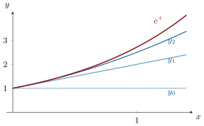
Run the machine on $y' = y$ , $y(0) = 1$ , starting from the constant $y^{(0)} \equiv 1$ : compute the Picard iterates $y^{(n)}$ , identify them, and describe the convergence.

Part III — Every hypothesis earns its keep.

(Lipschitz fails, uniqueness fails) For $y' = 2\sqrt{\abs y}$ , $y(0) = 0$ : check that $y \equiv 0$ and, for every $c \geq 0$ , the function $y_c(t) = 0$ for $t \leq c$ , $y_c(t) = (t - c)^2$ for $t > c$ , are all $C^1$ solutions on $\R$ . Where exactly does $y \mapsto 2\sqrt{\abs y}$ fail to be Lipschitz?
(Locality is real) For $y' = y^2$ , $y(0) = 1$ : solve explicitly, give the maximal interval of existence, and compute the best $h$ the theorem can certify over all choices of the rectangle ( $a$ large, $b$ free): show $h_{\max} = \sup_{b>0} \frac{b}{(1+b)^2} = \frac14$ , while the true solution lives on $\intoo{-\infty}{1}$ .
(Completeness is not decor) On $X = \Q \cap \intcc{1}{2}$ with the usual distance, let $g(x) = \frac x2 + \frac1x$ . Show $g(X) \subseteq X$ , that $g$ is a $\frac12$ -contraction (mean value inequality), and that $g$ has no fixed point in $X$ . Which hypothesis of Banach’s theorem fails, and what is the fixed point in the completion?
(Error bars) For a $k$ -contraction $g$ on a complete space, prove the a posteriori estimate $d(x_n, \ell) \leq \frac{k}{1-k}\,d(x_n, x_{n-1})$ . For Heron’s map $g(x) = \frac x2 + \frac 1x$ on $\intcc{1}{2}$ (fixed point $\sqrt2$ ), starting at $x_0 = \frac32$ : how many steps does the a priori bound $\frac{k^n}{1-k}d(x_1, x_0)$ demand for accuracy $10^{-6}$ , and how many steps suffice in reality? (Compute $x_1, x_2, x_3$ and their errors; the contraction bound is honest but pessimistic — Heron converges quadratically.)

Part IV — Continuous dependence. In this part $Lh < 1$ , so $T$ itself is a contraction on $X_h$ (question 7); write $y[\,y_0\,]$ for the solution with initial value $y_0$ .

(Dependence on the initial value) Let $z_0$ be another initial value with $\abs{z_0 - y_0}$ small enough that both problems fit in the rectangle. Using question 3, prove

$d_\infty\bigl(y[y_0], y[z_0]\bigr) \leq \frac{\abs{y_0 - z_0}}{1 - Lh}.$
(Long intervals by chaining) Suppose the solutions exist on a long segment cut into $m$ consecutive pieces on each of which the previous bound applies with $Lh \leq \frac12$ . Show the deviation grows by a factor at most $2$ per piece, hence $d_\infty \leq 2^m\abs{y_0 - z_0}$ overall — an exponential-in-length bound, the discrete shadow of the $\eu^{L\abs{t - t_0}}$ of Gronwall’s lemma (Chapter 16).
(Dependence on the field) Let $g$ be another field on $R$ , also $L$ -Lipschitz in $y$ , with $\sup_R \abs{f - g} \leq \varepsilon$ . Prove that the corresponding solutions satisfy $d_\infty \leq \frac{\varepsilon h}{1 - Lh}$ : modelling error propagates linearly.
(Parameters) If a family $f_\lambda$ of fields is $L$ -Lipschitz in $y$ uniformly and $\sup_R\abs{f_\lambda - f_\mu} \leq C\abs{\lambda - \mu}$ , deduce that $\lambda \mapsto y_\lambda$ is Lipschitz from the parameter space into $\bigl(C(I), d_\infty\bigr)$ .
(Systems cost nothing) Explain why Parts I, II and IV hold verbatim for $y$ with values in $\R^n$ (sup distances built on any of the distances of Example 4.2), then compute all Picard iterates for the system $y' = Ay$ , $y(0) = (c_1, c_2)$ , $A = \left(\begin{smallmatrix} 0 & 1\\ 0 & 0\end{smallmatrix}\right)$ : show the iteration becomes stationary at the exact solution after one step.

Part V — Metric dividends and synthesis.

(Perturbation of the identity) Let $X$ be a complete normed-space-like stage: take $X = C(I)$ or $\R^n$ . If $\eta \colon X \to X$ is $k$ -Lipschitz with $k < 1$ , prove that $x \mapsto x + \eta(x)$ is a bijection of $X$ whose inverse is $\frac1{1-k}$ -Lipschitz (for each $y$ , apply Banach to $x \mapsto y - \eta(x)$ ). This is the metric heart of the inverse function theorem (Chapter 15).
(Kepler’s equation) For $0 \leq e < 1$ and $m \in \R$ , prove that $x = m + e\sin x$ has exactly one solution, that the iteration $x_{n+1} = m + e\sin x_n$ converges to it from any start, and estimate: for $e = \frac12$ , $m = 1$ , how many iterations guarantee an error $\leq 10^{-3}$ by the a priori bound? (The solution is $x \approx 1.4987$ .)
(The Cantor set is a fixed point) Let $S_1(x) = \frac x3$ and $S_2(x) = \frac x3 + \frac23$ on $\R$ , and let $C$ be the Cantor set of Exercise 4.8. Prove $C = S_1(C) \cup S_2(C)$ , and explain in one sentence why no other nonempty compact set satisfies this equation (the map $A \mapsto S_1(A) \cup S_2(A)$ is a contraction for a distance between compact sets — the Hausdorff distance, made honest in the Year 3 volume).
(Connectedness globalizes uniqueness) Let $f$ be locally Lipschitz in $y$ on an open set, and let $y, z$ be two solutions of $y' = f(t, y)$ on a common interval $J$ with $y(t_0) = z(t_0)$ . Prove $y = z$ on $J$ : show that $\{t \in J : y(t) = z(t)\}$ is nonempty, closed in $J$ , and open in $J$ (by local uniqueness), and use the connectedness of intervals (Theorem 4.27).
(No smallness for linear equations) For $y' = \alpha(t)y + \beta(t)$ with $\alpha, \beta$ continuous on a segment $\intcc{A}{B}$ , adapt question 8 to show the factorial bound holds on the whole segment, so existence and uniqueness are global there — the scalar case of Chapter 16’s Cauchy–Lipschitz theorem, with no restriction on the length $B - A$ .
(Synthesis) One sentence each: what completeness contributed; what the contraction contributed; what the iterate trick bought compared with plain Banach; where connectedness entered; and which counterexample of Part III guards which hypothesis. Name the summit theorem, and say what replaces contraction when $f$ is merely continuous (Peano’s theorem, via compactness in function spaces — the Year 3 volume’s Arzelà–Ascoli).

Solution

Solution of Problem 4.1.

1. Let $F$ be closed in the complete $X$ and $(x_n) \subseteq F$ Cauchy: it converges in $X$ to some $\ell$ , and $\ell \in F$ because $F$ is closed (limits of sequences of $F$ stay in $\overline F = F$ ): $F$ is complete. Conversely let $A \subseteq X$ be complete and $x \in \overline A$ : some sequence of $A$ converges to $x$ ; it is Cauchy, so it converges in $A$ ; limits are unique, so $x \in A$ : $A$ closed. Since $\bigl(C(I), d_\infty\bigr)$ is complete (Theorem 4.9), its closed subsets are complete.

2. For $y, z \in C(I)$ and $t \in I$ :

\Bigl|\int_{t_0}^{t}y - \int_{t_0}^{t}z\Bigr| \leq \abs{t - t_0}\,\sup_I\abs{y - z} \leq h\,d_\infty(y, z),

and take the sup over $t$ .

3. Using the two fixed point equations and the triangle inequality:

d(\ell_g, \ell_{\widetilde g}) = d\bigl(g(\ell_g), \widetilde g(\ell_{\widetilde g})\bigr) \leq d\bigl(g(\ell_g), g(\ell_{\widetilde g})\bigr) + d\bigl(g(\ell_{\widetilde g}), \widetilde g(\ell_{\widetilde g})\bigr) \leq k\,d(\ell_g, \ell_{\widetilde g}) + d\bigl(g(\ell_{\widetilde g}), \widetilde g(\ell_{\widetilde g})\bigr),

and solve for $d(\ell_g, \ell_{\widetilde g})$ (the coefficient $1 - k$ is positive). The second inequality bounds the evaluated gap by the uniform one.

4. $g^m$ is a contraction on a nonempty complete space: it has a unique fixed point $\ell$ (Theorem 4.12). Then $g^m(g(\ell)) = g(g^m(\ell)) = g(\ell)$ : $g(\ell)$ is a fixed point of $g^m$ , so $g(\ell) = \ell$ by uniqueness. Any fixed point of $g$ is one of $g^m$ : uniqueness for $g$ . Orbits: fix $r \in \{0, \dots, m-1\}$ ; the subsequence $(x_{qm + r})_q$ is the $g^m$ -orbit started at $x_r$ , so it converges to $\ell$ as $q \to \infty$ (Banach again). All $m$ subsequences converge to the same $\ell$ , hence $x_n \to \ell$ : given $\varepsilon$ , each residue class is eventually within $\varepsilon$ , and there are finitely many classes.

5. If $y$ is continuous with values in $\intcc{y_0 - b}{y_0 + b}$ , the integrand $s \mapsto f(s, y(s))$ is continuous on $I$ (composition), so the right-hand side is $C^1$ with derivative $f(t, y(t))$ (fundamental theorem of calculus, Year 1 volume). If $y$ satisfies the integral equation, it is that $C^1$ function, $y(t_0) = y_0$ , and $y' = f(t, y)$ . Conversely, integrating $y' = f(s, y(s))$ from $t_0$ to $t$ gives the integral equation.

6. $X_h$ contains the constant $y_0$ ; it is closed as the preimage of $\intcc{0}{b}$ under the continuous map $y \mapsto d_\infty(y, y_0)$ (distances are $1$ -Lipschitz), hence complete by question 1. Stability: for $y \in X_h$ and $t \in I$ ,

\abs{T(y)(t) - y_0} = \Bigl|\int_{t_0}^{t}f(s, y(s))\dd s\Bigr| \leq M\abs{t - t_0} \leq Mh \leq b ,

the last step by $h \leq b/M$ (or $M = 0$ , trivial). And $T(y)$ is continuous ( $C^1$ even, question 5): $T(y) \in X_h$ .

7. For $t \in I$ :

\abs{T(y)(t) - T(z)(t)} \leq \int_{t_0}^{t}\abs{f(s, y(s)) - f(s, z(s))}\,\abs{\dd s} \leq L\abs{t - t_0}\,d_\infty(y,z) \leq Lh\,d_\infty(y,z).

If $Lh < 1$ : $T$ is a contraction of the nonempty complete $X_h$ , and Banach gives a unique fixed point — by question 5, the unique solution.

8. Induction; the case $n = 1$ is question 7’s middle inequality. Assuming the bound for $n$ , for $t \geq t_0$ (the case $t \leq t_0$ is symmetric):

\abs{T^{n+1}(y)(t) - T^{n+1}(z)(t)} \leq L\int_{t_0}^{t}\abs{T^n(y)(s) - T^n(z)(s)}\dd s \leq L\int_{t_0}^{t}\frac{L^n(s - t_0)^n}{n!}\dd s\; d_\infty(y,z),

and the integral evaluates to $\frac{L^n(t - t_0)^{n+1}}{(n+1)!}$ : the bound with $n + 1$ . Hence $d_\infty(T^n y, T^n z) \leq \frac{(Lh)^n}{n!}d_\infty(y, z)$ , and $\frac{(Lh)^n}{n!} \to 0$ (the exponential series converges): some $T^m$ is a contraction. Question 4 applies on the complete $X_h$ : $T$ has a unique fixed point, i.e. the Cauchy problem has exactly one solution on $I$ with values in $\intcc{y_0 - b}{y_0 + b}$ .

9. Let $y$ solve the problem on $I$ and suppose the set $E = \{t \in I, t > t_0 : \abs{y(t) - y_0} > b\}$ is nonempty (the side $t < t_0$ is symmetric); let $\tau = \inf E$ . By continuity, $\abs{y(s) - y_0} \leq b$ for $s \in \intcc{t_0}{\tau}$ , so the graph lies in $R$ there, the integral equation holds up to $\tau$ , and

\abs{y(\tau) - y_0} = \Bigl|\int_{t_0}^{\tau}f\bigl(s, y(s)\bigr)\dd s\Bigr| \leq M(\tau - t_0) \leq Mh \leq b .

If $\tau < t_0 + h$ , points of $E$ arbitrarily close to $\tau$ from the right give, by continuity, $\abs{y(\tau) - y_0} \geq b$ , hence $= b$ ; but then the display forces $M(\tau - t_0) = Mh$ , i.e. $\tau = t_0 + h$ : contradiction. So $\tau = t_0 + h$ , $E \subseteq \{t_0 + h\}$ , and the display (at $\tau = t_0 + h$ ) gives $\abs{y(t_0 + h) - y_0} \leq b$ , contradicting membership in $E$ . Hence $E = \emptyset$ : every solution on $I$ stays in the band, is a fixed point of $T$ in $X_h$ , and uniqueness is unconditional.

10. $T(y)(t) = 1 + \int_0^t y$ . From $y^{(0)} \equiv 1$ :

y^{(1)}(t) = 1 + t,\quad y^{(2)}(t) = 1 + t + \frac{t^2}2,\quad\dots\quad y^{(n)}(t) = \sum_{k=0}^{n}\frac{t^k}{k!}

(induction: integrating the partial sum adds the next term). These are the Taylor partial sums of $\eu^{\,t}$ ; on any bounded $I$ they converge uniformly to $\eu^{\,t}$ (the tail is dominated by the convergent numerical series $\sum h^k/k!$ ), which is indeed the unique solution.

11. $y \equiv 0$ is a solution. For $y_c$ : it is $C^1$ (both pieces are, and at $t = c$ the derivatives match: $0$ and $2(t - c) \to 0$ ), and for $t > c$ : $y_c' = 2(t - c) = 2\sqrt{(t-c)^2} = 2\sqrt{\abs{y_c}}$ ; for $t \leq c$ both sides vanish. So the Cauchy problem $y(0) = 0$ has infinitely many solutions ( $c \geq 0$ arbitrary, and $y \equiv 0$ ). The field $\varphi(y) = 2\sqrt{\abs y}$ is not Lipschitz near $0$ : $\frac{\varphi(y) - \varphi(0)}{y - 0} = \frac{2}{\sqrt y} \to +\infty$ as $y \to 0^+$ : no constant $L$ works on any neighbourhood of $0$ — exactly where all the solutions branch.

12. Separating variables (or checking directly), the unique local solution is $y(t) = \frac1{1 - t}$ , defined on $\intoo{-\infty}{1}$ and blowing up at $t = 1$ . For the rectangle $\intcc{-a}{a} \times \intcc{1 - b}{1 + b}$ : $M = \sup y^2 = (1 + b)^2$ , so the certified half-width is $h = \min\bigl(a, \frac{b}{(1+b)^2}\bigr)$ . Maximizing $\frac{b}{(1+b)^2}$ : derivative zero at $b = 1$ , value $\frac14$ . So the theorem guarantees life only on $\intcc{-\frac14}{\frac14}$ — correctly less than the true lifespan $1$ forward, and infinitely less backward: the theorem is local by nature, and blow-up shows it cannot be otherwise.

13. $g$ maps $\intcc12$ into itself: $g$ decreases on $\intcc{1}{\sqrt2}$ and increases after (study $g'(x) = \frac12 - \frac1{x^2}$ ), with $g(1) = g(2) = \frac32$ and minimum $g(\sqrt2) = \sqrt2 > 1$ : $g(\intcc12) \subseteq \intcc{\sqrt2}{\frac32} \subseteq \intcc12$ ; and $g$ maps rationals to rationals. Contraction: $\abs{g'(x)} = \abs{\frac12 - \frac1{x^2}} \leq \frac12$ on $\intcc12$ ( $\frac1{x^2} \in \intcc{\frac14}{1}$ ), so the mean value inequality gives $\abs{g(x) - g(y)} \leq \frac12\abs{x - y}$ . A fixed point satisfies $\frac x2 = \frac1x$ , i.e. $x^2 = 2$ : impossible in $\Q$ . The failing hypothesis is completeness of $X$ ( $\Q \cap \intcc12$ is not complete); in the completion $\intcc12$ the fixed point is $\sqrt2$ — Banach’s theorem run on the rationals creates the irrational.

14. A posteriori: $d(x_n, \ell) \leq d(x_n, x_{n+1}) + d(x_{n+1}, \ell) \leq k\,d(x_{n-1}, x_n) + k\,d(x_n, \ell)$ , whence $d(x_n, \ell) \leq \frac{k}{1-k}d(x_n, x_{n-1})$ . Heron from $x_0 = \frac32$ : $x_1 = \frac{17}{12}$ , $d(x_1, x_0) = \frac1{12}$ , $k = \frac12$ : the a priori bound $\frac{k^n}{1-k}d(x_1,x_0) = \frac{2^{-n+1}}{12}$ drops below $10^{-6}$ first at $n = 18$ . In reality $x_1 = \frac{17}{12} \approx 1.41667$ (error $2.5\cdot10^{-3}$ ), $x_2 = \frac{577}{408} \approx 1.4142157$ (error $2.1\cdot10^{-6}$ ), $x_3 \approx 1.41421356237469$ (error $1.6\cdot10^{-12}$ ): three steps suffice. Each Heron step roughly squares the error (quadratic convergence, a Newton phenomenon: Chapter 8); the contraction estimate, which only halves it, is honest for the worst case but pessimistic here.

15. Apply question 3 with $g = T_{y_0}$ (an $Lh$ -contraction, $Lh < 1$ ) and $\widetilde g = T_{z_0}$ , whose fixed point is $y[z_0]$ . For any $y$ ,

\abs{T_{y_0}(y)(t) - T_{z_0}(y)(t)} = \abs{y_0 - z_0},

(the integrals are identical), so $\sup_y d_\infty(T_{y_0}(y), T_{z_0}(y)) = \abs{y_0 - z_0}$ , and question 3 gives

d_\infty(y[y_0], y[z_0]) \leq \frac{\abs{y_0 - z_0}}{1 - Lh} .

16. On each piece, question 15 applied with the left-endpoint values as initial data bounds the deviation at the right endpoint:

d_\infty \leq \frac{1}{1 - 1/2}\,(\text{left deviation}) = 2\,(\text{left deviation}) .

By induction over the $m$ pieces, the final deviation is at most $2^m\abs{y_0 - z_0}$ , and the uniform deviation over the whole segment obeys the same bound (each piece’s sup is controlled at its stage). With pieces of length $h \asymp \frac1{2L}$ , the factor is $2^m = 2^{\,\text{length}\cdot 2L}$ : exponential in the length of the interval, exactly as Gronwall’s bound $\eu^{L\abs{t-t_0}}$ predicts, with better constants.

17. Same scheme: for $y \in X_h$ ,

\abs{T_f(y)(t) - T_g(y)(t)} \leq \int_{t_0}^t \abs{f(s,y(s)) - g(s,y(s))}\,\abs{\dd s} \leq \varepsilon h ,

so question 3 (with $T_f$ the contraction, $T_g$ the perturbed map) yields $d_\infty \leq \frac{\varepsilon h}{1 - Lh}$ .

18. By question 17 applied to $f = f_\lambda$ , $g = f_\mu$ : $d_\infty(y_\lambda, y_\mu) \leq \frac{Ch}{1 - Lh}\abs{\lambda - \mu}$ : the solution map is Lipschitz with constant $\frac{Ch}{1-Lh}$ .

19. Every argument used only: the metric axioms, the completeness of the stage, the bound $\abs{\int} \leq \int\abs{\cdot}$ , and the Lipschitz property of $f$ — all available for $\R^n$ -valued functions with $d_\infty$ built on any of the equivalent distances of Example 4.2 (complete by Theorem 4.9). For $y' = Ay$ with the nilpotent $A$ : $y^{(0)} \equiv (c_1, c_2)$ ,

y^{(1)}(t) = (c_1, c_2) + \int_0^t (c_2, 0)\,\dd s = (c_1 + tc_2,\; c_2),

and $Ay^{(1)}(s) = (c_2, 0)$ again: $y^{(2)} = y^{(1)}$ . The iteration is stationary from $n = 1$ on, at the exact solution $y(t) = (c_1 + tc_2, c_2) = \eu^{tA}y(0)$ — nilpotency truncates the exponential series, and Picard notices.

20. Fix $y \in X$ and let $g_y(x) = y - \eta(x)$ : a $k$ -contraction of the complete $X$ , so there is exactly one $x$ with $x + \eta(x) = y$ : the map $\Phi = \mathrm{id} + \eta$ is bijective. Lipschitz inverse: if $\Phi(x) = y$ and $\Phi(x') = y'$ ,

d(x, x') \leq d(y, y') + d\bigl(\eta(x), \eta(x')\bigr) \leq d(y, y') + k\,d(x, x'),

so $d(x, x') \leq \frac{1}{1-k}d(y, y')$ . (Distances here come from the norm structure, so $d(a - c, b - c) = d(a, b)$ , which the first inequality used.)

21. $g(x) = m + e\sin x$ is $e$ -Lipschitz on the complete $\R$ (mean value inequality, $\abs{g'} = \abs{e\cos x} \leq e < 1$ ): Banach gives a unique solution and global convergence of the iteration. For $e = \frac12$ , $m = 1$ , $x_0 = 1$ : $x_1 = 1 + \frac12\sin 1 \approx 1.42074$ , $d(x_1, x_0) \approx 0.4207$ , and the a priori bound $\frac{(1/2)^n}{1/2}\cdot 0.4207 \leq 10^{-3}$ first holds at $n = 10$ : ten iterations certified (the true value $x \approx 1.4987$ is in fact reached to $10^{-3}$ already around $n = 5$ ).

22. Use the digit description (Exercise 4.8): $C$ is the set of sums $\sum_{n\geq1}a_n3^{-n}$ , $a_n \in \{0, 2\}$ . Then $S_1(C) = \{x/3 : x \in C\}$ is the subset with $a_1 = 0$ , and $S_2(C) = \{x/3 + 2/3\}$ the subset with $a_1 = 2$ : their union, over the free choice of $a_1$ , is exactly $C$ . Uniqueness in one sentence: on the space of nonempty compact subsets of $\intcc01$ metrized by the Hausdorff distance, $A \mapsto S_1(A) \cup S_2(A)$ is a $\frac13$ -contraction of a complete space, so Banach allows only one fixed set — the Year 3 volume makes the Hausdorff metric and this argument rigorous.

23. Let $Z = \{t \in J : y(t) = z(t)\}$ : nonempty ( $t_0 \in Z$ ), closed in $J$ (equalizer of two continuous maps: preimage of $\{0\}$ under $y - z$ ). Open: if $t_1 \in Z$ , apply the local theorem (question 8) at the point $(t_1, y(t_1))$ , in a rectangle where $f$ is Lipschitz: on a small interval around $t_1$ both $y$ and $z$ solve the same Cauchy problem, so they coincide there (question 9’s unconditional uniqueness): a neighbourhood of $t_1$ lies in $Z$ . A nonempty subset of the interval $J$ that is both open and closed in $J$ is all of $J$ (intervals are connected, Theorem 4.27): $y = z$ on $J$ .

24. Here $f(t, y) = \alpha(t)y + \beta(t)$ is $L$ -Lipschitz in $y$ on all of $\intcc AB \times \R$ with $L = \sup\abs\alpha$ (finite: $\alpha$ continuous on a segment), and no band $\intcc{y_0 - b}{y_0 + b}$ is needed: take $X = C(\intcc AB)$ entire, on which $T$ is well defined. The induction of question 8 runs verbatim and gives $d_\infty(T^ny, T^nz) \leq \frac{(L(B - A))^n}{n!}d_\infty(y, z)$ : an iterate is a contraction whatever the length $B - A$ , and question 4 concludes: one and only one solution on the whole segment. Linearity enters exactly once: it makes the Lipschitz bound global in $y$ , removing the rectangle and its $h \leq b/M$ .

25. Completeness turned the Cauchy sequence of iterates into an actual solution (questions 1, 6, 8), and its absence let $\sqrt2$ escape from $\Q$ (question 13). Contraction gave uniqueness, the algorithm, and the error bars (questions 7, 14). The iterate trick removed the smallness condition $Lh < 1$ , so the certified interval depends only on $M$ , not on $L$ — and made linear equations global (questions 8, 24). Connectedness promoted local uniqueness to global uniqueness (question 23). The counterexamples: $2\sqrt{\abs y}$ guards Lipschitz (question 11), $y^2$ guards locality (question 12), $\Q$ guards completeness (question 13). The summit is the Picard–Lindelöf theorem (question 8); when $f$ is merely continuous, existence survives but uniqueness dies, and the proof trades the contraction for compactness of function sets — Peano’s theorem via Arzelà–Ascoli, in the Year 3 volume.