Definition 32.1High School Mathematics · Chapter 32 — Conditional Probability and Independence
Let B be an event with P(B)>0. The probability of A given B is
PB(A)=P(B)P(A∩B).
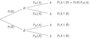
A two-level tree: multiply along a path, add over the leaves. For instance P(A) is the sum of the first and third leaf probabilities.
Examples
Example 32.6(Screening test)
A disease affects 1% of a population. A test detects it with probability0.99 (sensitivity) and gives a false positive with probability0.05. Given a positive test, the probability of actually having the disease is
Despite the accurate test, five positives out of six are false — because the disease is rare. Confusing PA(B) with PB(A) is the prosecutor’s fallacy.
Read in context →
Definition 21.10University Mathematics — Year 2 · Chapter 21 — Probability on Countable Spaces
For eventsA,B with P(B)>0, the conditional probability of A given B is
Roll two fair dice and condition on the sum being 7: for each k∈[[1,6]],
P{S=7}(X=k)=P(S=7)P(X=k,Y=7−k)=6/361/36=61:
given a sum of 7, the first die is exactly uniform — 7 is the only total compatible with every face, so the conditioning erases all information about X. Any other total skews the law (given S=4, the first die is uniform on {1,2,3} only). Computing a conditional law means renormalizing the joint weights along the conditioning event, nothing more.
Example 21.13(The second draw is as good as the first)
An urn holds 3 white and 2 black balls; draw two without replacement. Everyone agrees P(W1)=53; what is P(W2)? Total probability along the first draw:
exactly P(W1). No computation was needed: by symmetry, every ball is equally likely to be the second one drawn, so the second draw — unconditionally — has the same law as the first. Conditioning on the first result changes the odds; not knowing it does not. This exchangeability argument returns in the next chapter for sampling without replacement, where it gives the hypergeometric mean np with no binomial identities at all.
Example 21.15(The birthday collision, by the chain rule)
With n people whose birthdays are independent and uniform over 365 days, let Dn=“all n birthdays differ”. Conditioning person by person (chain rule):
P(Dn)=k=1∏n−1(1−365k),
each new person having to avoid the k days already taken. For n=23: P(D23)≈0.493 — a shared birthday is already more likely than not. The heuristic that explains the smallness of 23: taking logarithms, −lnP(Dn)≈∑k<n365k=365(2n), and (223)=253 gives 253/365≈0.693≈ln2. What matters is the number of pairs, which grows quadratically: collision problems live on the scale n∼365, not n∼365 — the birthday paradox is a square root in disguise.
 Coach
Coach