High School Mathematics · Grades 10–12

9Probability and Sampling

Probability assigns numbers to chance. Starting from experiments with equally likely outcomes — dice, coins, cards — this chapter builds the basic rules for computing probabilities of events, introduces tree diagrams for two-step experiments, and ends with the link between probabilities and observed frequencies. The theory continues in Chapter 18.

9.1 Random experiments and events

Definition 9.1 (Outcomes and events)

A random experiment is an experiment whose result cannot be predicted (rolling a die). The set of all possible results is the sample space $\Omega = \{\omega_1, \dots, \omega_n\}$ ; its elements are the outcomes. An event is a set of outcomes; an event occurs when the result of the experiment belongs to it.

Definition 9.2 (Probability distribution)

Assigning to each outcome $\omega_i$ a number $p_i \geq 0$ , with $p_1 + \dots + p_n = 1$ , defines a probability: the probability $\P(A)$ of an event $A$ is the sum of the $p_i$ of the outcomes in $A$ . In particular $\P(\Omega) = 1$ and the impossible event $\varnothing$ has probability $0$ .

Proposition 9.3 (Equally likely outcomes)

If the $n$ outcomes are equally likely (each $p_i = \frac1n$ ), then for every event $A$ :

\P(A) = \frac{\text{number of outcomes in } A}{n} = \frac{\text{favorable cases}}{\text{possible cases}} .

Proof. $A$ contains some number $k$ of outcomes, each of probability $\frac1n$ , so $\P(A) = \frac kn$ . ∎

Example 9.4

Roll a fair die: $\Omega = \{1, 2, 3, 4, 5, 6\}$ , each outcome having probability $\frac16$ . The event $A$ : “the result is even” is $A = \{2, 4, 6\}$ , so $\P(A) = \frac36 = \frac12$ . The event $B$ : “the result is at least $5$ ” is $B = \{5, 6\}$ , so $\P(B) = \frac26 = \frac13$ .

9.2 Combining events

Definition 9.5 (Intersection, union, complement)

Let $A$ and $B$ be events.

$A \cap B$ (“ $A$ and $B$ ”) occurs when both occur;
$A \cup B$ (“ $A$ or $B$ ”) occurs when at least one occurs;
the complement $\bar A$ (“not $A$ ”) occurs exactly when $A$ does not;
$A$ and $B$ are incompatible when they cannot occur together: $A \cap B = \varnothing$ .

Theorem 9.6 (Addition rules)

For all events $A$ and $B$ :

\P(A \cup B) = \P(A) + \P(B) - \P(A \cap B), \qquad \P(\bar A) = 1 - \P(A) .

For incompatible events, the first rule simplifies to $\P(A \cup B) = \P(A) + \P(B)$ .

Proof. Summing $\P(A) + \P(B)$ adds the probability of every outcome of $A \cup B$ once, except those of $A \cap B$ , which are counted twice — once in $A$ and once in $B$ . Subtracting $\P(A \cap B)$ repairs the double counting. For the complement: $A$ and $\bar A$ are incompatible and $A \cup \bar A = \Omega$ , so $\P(A) + \P(\bar A) = \P(\Omega) = 1$ . ∎

Two overlapping events: in (A) + (B), the shaded intersection A ∩ B is counted twice, which explains the subtraction in the addition rule. — Two overlapping events: in $\P(A) + \P(B)$ , the shaded intersection $A \cap B$ is counted twice, which explains the subtraction in the addition rule.

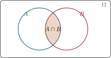
Example 9.7

Draw one card from a standard $52$ -card deck. Let $A$ : “the card is a heart” ( $13$ cards) and $B$ : “the card is a king” ( $4$ cards). Then $A \cap B$ is “the king of hearts” ( $1$ card), and

\P(A \cup B) = \frac{13}{52} + \frac{4}{52} - \frac{1}{52} = \frac{16}{52} = \frac{4}{13}.

The complement rule is often the fastest route: the probability that the card is not a heart is $1 - \frac{13}{52} = \frac34$ .

9.3 Tree diagrams

Method 9.8 (Two-step experiments)

For an experiment performed in two steps:

draw a tree: one branch per possible result of the first step, then from each of these, one branch per result of the second step, writing the probability on each branch (the branches leaving any node must sum to $1$ );
the probability of a path (a leaf of the tree) is the product of the probabilities along its branches;
the probability of an event is the sum of the probabilities of the paths that realize it.

Example 9.9

An urn contains $3$ red balls and $2$ blue balls. Draw one ball, put it back, draw again. Each draw gives red (R) with probability $\frac35$ and blue (B) with probability $\frac25$ .

The tree of two draws with replacement. The four path probabilities sum to 1. — The tree of two draws with replacement. The four path probabilities sum to $1$ .

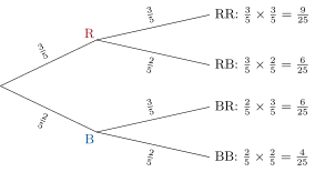
The probability of getting two balls of the same color is $\P(\text{RR}) + \P(\text{BB}) = \frac{9}{25} + \frac{4}{25} = \frac{13}{25}$ ; the probability of at least one blue is $1 - \P(\text{RR}) = 1 - \frac{9}{25} = \frac{16}{25}$ (complement rule).

Remark 9.10

Without replacement, the probabilities of the second draw depend on the first: with the urn above, after drawing a red ball, only $2$ red and $2$ blue remain, so the second branch carries $\frac24$ and $\frac24$ . The tree method works unchanged; only the numbers on the second-level branches change.

9.4 Frequencies and sampling

When a random experiment is repeated many times, the observed frequency of an event approaches its probability — this is why probability is useful for describing the real world.

Definition 9.11 (Sample)

A sample of size $n$ is the result of repeating the same experiment $n$ times independently. The observed frequency of an event in the sample is the number of occurrences divided by $n$ .

Example 9.12

A fair coin gives heads with probability $0.5$ . Tossing it $100$ times rarely gives exactly $50$ heads: samples fluctuate. Typical runs of $100$ tosses give frequencies like $0.46$ , $0.53$ , $0.49$ — close to $0.5$ , but not equal. Larger samples fluctuate less: with $10\,000$ tosses, observed frequencies are usually within about $0.01$ of $0.5$ .

Remark 9.13 (Fluctuation interval)

A useful rule of thumb, justified in Chapter 19: for a sample of size $n$ of an event of probability $p$ (with $n$ reasonably large), the observed frequency lies in the interval

\intcc{p - \frac{1}{\sqrt n}}{\,p + \frac{1}{\sqrt n}}

in roughly $95\%$ of samples. If an observed frequency falls far outside this interval, doubt the value of $p$ : this is the starting point of statistical testing.

Example 9.14

A factory claims that only $10\%$ of its parts are defective ( $p = 0.1$ ). In a sample of $n = 400$ parts, $64$ are defective: observed frequency $\frac{64}{400} = 0.16$ . The fluctuation interval is $\intcc{0.1 - \frac{1}{20}}{0.1 + \frac{1}{20}} = \intcc{0.05}{0.15}$ , and $0.16$ falls outside it: the sample casts serious doubt on the claim.

9.5 Exercises

Exercise 9.1 ★

A fair die is rolled. Compute the probability of each event: “getting a $6$ ”; “getting an odd number”; “getting at most $4$ ”; “getting a $7$ ”.

Solution

Solution of Exercise 9.1.

Each of the $6$ outcomes has probability $\frac16$ . “Getting a $6$ ”: $\frac16$ . “Odd number” $= \{1, 3, 5\}$ : $\frac36 = \frac12$ . “At most $4$ ” $= \{1,2,3,4\}$ : $\frac46 = \frac23$ . “Getting a $7$ ”: impossible event, probability $0$ .

Exercise 9.2 ★

A bag contains $5$ green, $3$ yellow and $2$ black marbles; one marble is drawn at random. Compute the probability that it is green; that it is not black; that it is green or yellow.

Solution

Solution of Exercise 9.2.

There are $10$ equally likely marbles. $\P(\text{green}) = \frac{5}{10} = \frac12$ . $\P(\text{not black}) = 1 - \frac{2}{10} = \frac{8}{10} = \frac45$ . Green and yellow are incompatible: $\P(\text{green or yellow}) = \frac{5}{10} + \frac{3}{10} = \frac{8}{10} = \frac45$ .

Exercise 9.3 ★

In a class of $30$ students, $18$ study Spanish, $10$ study German, and $4$ study both. A student is picked at random. Using the addition rule, compute the probability that this student studies at least one of the two languages, then the probability that they study neither.

Solution

Solution of Exercise 9.3.

Let $S$ : “studies Spanish”, $G$ : “studies German”. Then $\P(S) = \frac{18}{30}$ , $\P(G) = \frac{10}{30}$ , $\P(S \cap G) = \frac{4}{30}$ . Addition rule:

\P(S \cup G) = \frac{18}{30} + \frac{10}{30} - \frac{4}{30} = \frac{24}{30} = \frac45 .

Complement: $\P(\text{neither}) = 1 - \frac45 = \frac15$ .

Exercise 9.4 ★

A fair coin is tossed twice. Draw the tree of the experiment and compute the probability of getting two heads; exactly one head; at least one head.

Solution

Solution of Exercise 9.4.

The tree has four paths HH, HT, TH, TT, each of probability $\frac12 \times \frac12 = \frac14$ . Two heads: $\frac14$ . Exactly one head (HT or TH): $\frac24 = \frac12$ . At least one head: $1 - \P(\text{TT}) = 1 - \frac14 = \frac34$ .

Exercise 9.5 ★★

An urn contains $4$ red and $6$ white balls. Two balls are drawn one after the other without replacement. Draw the tree with the correct probabilities on the second level, and compute the probability of drawing two red balls, then of drawing two balls of different colors.

Solution

Solution of Exercise 9.5.

First draw: red with probability $\frac{4}{10}$ , white $\frac{6}{10}$ . Second draw without replacement: after a red, $3$ red and $6$ white remain among $9$ ; after a white, $4$ red and $5$ white among $9$ .

Two reds: $\frac{4}{10} \times \frac39 = \frac{12}{90} = \frac{2}{15}$ .

Different colors: paths RW and WR:

\frac{4}{10} \times \frac69 + \frac{6}{10} \times \frac49 = \frac{24}{90} + \frac{24}{90} = \frac{48}{90} = \frac{8}{15}.

Exercise 9.6 ★★

Two fair dice are rolled and their sum is recorded.

Explain why the sample space can be taken as the $36$ equally likely pairs $(1,1), (1,2), \dots, (6,6)$ .
Compute the probability that the sum is $7$ ; that it is $12$ ; that it is at most $4$ .
Which sum is the most likely?

Solution

Solution of Exercise 9.6.

1. Each die independently shows each face with probability $\frac16$ , so the $36$ ordered pairs are equally likely; the sum is determined by the pair.

2. Sum $7$ : the pairs $(1,6), (2,5), (3,4), (4,3), (5,2), (6,1)$ , so $\P = \frac{6}{36} = \frac16$ . Sum $12$ : only $(6,6)$ , $\P = \frac{1}{36}$ . Sum at most $4$ : pairs summing to $2$ , $3$ or $4$ : $(1,1)$ ; $(1,2), (2,1)$ ; $(1,3), (2,2), (3,1)$ — six pairs, so $\P = \frac{6}{36} = \frac16$ .

3. The number of pairs achieving each sum grows from $1$ (sum $2$ ) to $6$ (sum $7$ ) then decreases: the most likely sum is $7$ .

Exercise 9.7 ★★

A multiple-choice question offers $4$ answers, one correct. A student answers $2$ independent such questions completely at random. Compute the probability of answering both correctly, exactly one correctly, none correctly. Check that the three probabilities sum to $1$ .

Solution

Solution of Exercise 9.7.

Each question is answered correctly with probability $\frac14$ , independently. Tree with two levels:

Both correct: $\frac14 \times \frac14 = \frac{1}{16}$ .

Exactly one correct: paths correct–wrong and wrong–correct: $\frac14 \times \frac34 + \frac34 \times \frac14 = \frac{6}{16} = \frac38$ .

None correct: $\frac34 \times \frac34 = \frac{9}{16}$ .

Check: $\frac{1}{16} + \frac{6}{16} + \frac{9}{16} = 1$ .

Exercise 9.8 ★★

A politician claims $50\%$ approval. In a poll of $n = 900$ randomly chosen voters, $396$ approve.

Compute the observed frequency and the fluctuation interval around $p = 0.5$ for $n = 900$ .
Does the poll cast doubt on the claim?

Solution

Solution of Exercise 9.8.

1. Observed frequency: $\frac{396}{900} = 0.44$ . With $n = 900$ : $\frac{1}{\sqrt{900}} = \frac{1}{30} \approx 0.033$ , so the fluctuation interval is about $\intcc{0.467}{0.533}$ .

2. The observed $0.44$ lies outside the interval: samples of $900$ voters from a population with $50\%$ approval rarely stray that far. The poll casts serious doubt on the claimed $50\%$ .

Exercise 9.9 ★★★

A game costs $2$ to play: you roll a fair die and win $6$ if you roll a $6$ , $3$ if you roll a $5$ , nothing otherwise.

Compute the probability of each amount won ( $6$ , $3$ , $0$ ).
Over $600$ games, about how many of each outcome do you expect? Compute the total expected gain and loss: is the game worth playing?

Solution

Solution of Exercise 9.9.

1. $\P(\text{win } 6) = \frac16$ (roll a $6$ ), $\P(\text{win } 3) = \frac16$ (roll a $5$ ), $\P(\text{win } 0) = \frac46 = \frac23$ .

2. Over $600$ games, expect about $100$ sixes, $100$ fives, $400$ other rolls. Winnings: about $100 \times 6 + 100 \times 3 = 900$ . Cost: $600 \times 2 = 1200$ . Expected net result: $900 - 1200 = -300$ , i.e. a loss of about $0.5$ per game on average — the game is not worth playing.

9.6 Problem: The three doors that fooled a thousand mathematicians

Problem 9.1

Weekend problem — the Monty Hall paradox and its cousins: how information changes probability, and how samples separate claims from wishful thinking

In 1990 the columnist Marilyn vos Savant published a puzzle about a game show host, three doors, a car and two goats — and answered it correctly. Ten thousand readers, among them hundreds of mathematics PhDs, wrote in to insist she was wrong. This problem arms you with trees (Method 9.8), complements and the addition rules (Theorem 9.6), lets you settle the argument yourself, and finishes with the tool that arbitrates every such dispute in practice: the fluctuating sample.

Part I — The rules, warmed up.

One card from a standard $52$ -card deck: compute $P(\text{king or heart})$ with the addition rule — and say why $\frac{4}{52} + \frac{13}{52}$ alone is wrong.
Three fair coin flips: compute $P(\text{at least one head})$ by the complement.
A bag holds $3$ red and $2$ blue marbles; two are drawn without replacement. With a tree, compute $P(\text{two reds})$ and $P(\text{one of each color})$ .
Complete the distribution of question 3 with $P(\text{two blues})$ and check the three probabilities sum to $1$ .
Someone reports, for two incompatible events, $P(A) = 0.6$ and $P(B) = 0.5$ . Convict them with one line of arithmetic.

Part II — The three doors. The game: a car hides behind one of three doors, goats behind the other two. You pick a door (say door 1). The host — who knows where the car is — opens one of the other two doors, always revealing a goat, and offers you the chance to switch to the remaining closed door.

Before computing anything: does switching help, hurt, or not matter? Write down your gut answer — honestly.
Now the tree, by cases on the car’s true position (each $\frac13$ ): if the car is behind your door, switching loses; if it is behind either other door, what must the host do, and what does switching then win? Compute $P(\text{win by switching})$ .
The one-line version: switching wins exactly when your first pick was wrong. Conclude again.
Now the crucial variant — “Monty Fall”: the host does not know where the car is, opens one of the other doors at random, and by luck reveals a goat. List the six equally likely scenarios (car position $\times$ door opened), discard those where the car is revealed, and compute the probability that switching wins among the surviving scenarios. What changed, and why does the host’s knowledge matter?
The intuition pump: one hundred doors, you pick one, the knowing host opens $98$ goat doors. Switch? With what probability of winning?
You face a skeptic who, like the thousand letter-writers, insists on “50–50”. Describe a card-based simulation (three cards, many rounds, a friend as host) and say what proportion of switching wins you expect after $300$ rounds — with the fluctuation interval of the chapter as your margin.

Part III — Cousins of the paradox.

A family has two children; you learn that at least one is a boy. List the equally likely two-children configurations compatible with the information, and compute $P(\text{two boys})$ .
Same family, but the information is now: the elder child is a boy. Recompute. Why do the two answers differ, and what do they share with the two Montys?
Three fair coins: compute $P(\text{all three alike})$ . The mathematician d’Alembert argued in 1754 for another answer: “either they are all alike or they are not — one case in two.” Name the exact error, with Proposition 9.3 in hand.
A game costs $2$ euros: roll a die, win $6$ euros on a six, $3$ euros on a five, nothing otherwise (Exercise 9.9). Over $600$ games, what average gain per game does the counting predict? An insurer plays the same mathematics: a $1\,\%$ yearly chance of a $10\,000$ -euro claim — what is the fair premium, and why does the real premium exceed it?

Part IV — Samples as arbiters.

A coin is flipped $100$ times. Using the fluctuation interval $p \pm \frac{1}{\sqrt n}$ , decide which of these outcomes should raise eyebrows: $55$ heads; $70$ heads.
A poll of $1\,000$ voters gives a candidate $52\,\%$ . Compute the fluctuation interval around $50\,\%$ and say whether the poll proves the candidate is ahead.
A factory claims $4\,\%$ defective parts. A sample of $400$ shows $28$ defective ( $7\,\%$ ); a later sample of $2\,500$ shows $175$ ( $7\,\%$ again). Test the claim against each sample. Why do the verdicts differ?
Two error sources haunt every survey: sampling bias (the how-data-lies weekend problem of the Middle School volume) and sampling fluctuation (this chapter). Which one shrinks as $n$ grows, and which one survives any sample size? One sentence each.
Finale — the probabilist’s checklist, one line per item: outcomes equally likely before counting (question 15); trees and complements for multi-step and “at least” (questions 2–3); information changes probabilities, and how it was obtained matters (questions 7–14); samples fluctuate by about $\frac{1}{\sqrt n}$ , and simulation arbitrates (questions 11, 16–18).

Solution

Solution of Problem 9.1.

1. $P(\text{king or heart}) = \frac{4}{52} + \frac{13}{52} - \frac{1}{52} = \frac{16}{52} = \frac{4}{13}$ : the king of hearts sits in both events and must not be counted twice — hence the subtraction (Theorem 9.6).

2. $P(\text{no head}) = \left(\frac12\right)^3 = \frac18$ , so $P(\text{at least one}) = \frac78$ .

3. $P(RR) = \frac35 \times \frac24 = \frac{3}{10}$ ; $P(\text{one of each}) = \frac35 \times \frac24 + \frac25 \times \frac34 = \frac{6}{20} + \frac{6}{20} = \frac35$ .

4. $P(BB) = \frac25 \times \frac14 = \frac1{10}$ ; and $\frac{3}{10} + \frac{6}{10} + \frac{1}{10} = 1$ : the tree’s leaves always total $1$ .

5. Incompatible events obey $P(A \cup B) = P(A) + P(B) = 1.1 > 1$ : impossible — some probability was invented.

6. (Most people, including the thousand letter-writers, answer “it doesn’t matter, 50–50”. Keep your answer for question 8.)

7. Car behind door 1 (probability $\frac13$ ): the host opens either goat door; switching leaves the car: lose. Car behind door 2 ( $\frac13$ ): the host must open door 3; switching lands on door 2: win. Car behind door 3: symmetric: win. Total: $P(\text{switch wins}) = \frac13 + \frac13 = \frac23$ .

8. Your first pick is wrong with probability $\frac23$ — and precisely then, the host’s forced reveal leaves the car behind the remaining door: switching converts every initial error into a win. $\frac23$ , whatever the gut said.

9. Six equally likely scenarios: car behind $1$ , $2$ or $3$ , host opens door $2$ or $3$ (never yours). The reveal shows the car in two of them (car@2/opens 2, car@3/opens 3): discarded. Among the four survivors — car@1/opens 2, car@1/opens 3, car@2/opens 3, car@3/opens 2 — switching wins in the last two: $\frac24 = \frac12$ . With an ignorant host, 50–50 is correct: the paradox lives entirely in the host’s knowledge, which filters the scenarios unevenly.

10. Your pick holds the car with probability $\frac{1}{100}$ ; the knowing host’s $98$ reveals funnel the remaining $\frac{99}{100}$ onto the one closed door. Switch, and win $99$ times in $100$ .

11. Three cards (one ace, two jokers), a friend who peeks and always discards a joker from the two you did not pick; play $300$ rounds, always switching, and record wins. Expected frequency $\frac23 \approx 0.667$ , with fluctuation $\pm\frac{1}{\sqrt{300}} \approx 0.058$ : expect between about $61\,\%$ and $72\,\%$ switching wins — far from any “50–50”.

12. Equally likely configurations (elder–younger): BB, BG, GB, GG. “At least one boy” keeps BB, BG, GB: $P(\text{BB}) = \frac13$ .

13. “The elder is a boy” keeps BB, BG: $P(\text{BB}) = \frac12$ . Different information filters different scenario sets — exactly as the two Montys did: what you learn matters, and how you learned it matters just as much.

14. All alike: HHH, TTT: $\frac28 = \frac14$ . D’Alembert’s error: his two “cases” are not equally likely — “not all alike” bundles six of the eight outcomes. Proposition 9.3 counts only over equally likely outcomes.

15. Average winnings per game: $6 \times \frac16 + 3 \times \frac16 = 1.50$ euros, against a $2$ -euro stake: an average loss of $0.50$ per game, about $300$ euros over $600$ games. The fair premium equalizes average payout: $1\,\% \times 10\,000 = 100$ euros; real premiums add costs and a safety margin — the insurer must survive bad years, not just average ones.

16. Interval: $0.5 \pm \frac{1}{\sqrt{100}} = \intcc{0.4}{0.6}$ . $55$ heads ( $0.55$ ): inside, unremarkable. $70$ heads ( $0.70$ ): far outside — doubt the coin.

17. $\frac{1}{\sqrt{1000}} \approx 0.032$ : a fair $50\,\%$ candidate would typically poll in $\intcc{0.468}{0.532}$ — and $0.52$ sits comfortably inside. The poll suggests a lead but proves nothing: the margin swallows it.

18. First sample: interval $0.04 \pm \frac{1}{20} = \intcc{0}{0.09}$ ; the observed $0.07$ is inside: no verdict. Second: $0.04 \pm \frac{1}{50} = \intcc{0.02}{0.06}$ ; the observed $0.07$ falls outside: the claim is now in serious doubt. Same frequency, sharper instrument: precision grows like $\sqrt n$ .

19. Fluctuation shrinks like $\frac{1}{\sqrt n}$ : quadruple the sample, halve the noise. Bias — asking the wrong crowd — survives any $n$ : two million badly chosen ballots stayed wrong (the how-data-lies weekend problem of the Middle School volume).

20. (i) Check outcomes are equally likely before counting — d’Alembert forgot. (ii) Trees multiply along branches; “at least one” surrenders to the complement. (iii) Information filters scenarios, and its source changes the filter — knowing Monty against fallen Monty, elder-boy against some-boy. (iv) Frequencies approach probabilities at speed $\frac{1}{\sqrt n}$ , so a patient simulation settles any argument — including one with ten thousand angry letter-writers.