High School Mathematics · Grades 10–12

32Conditional Probability and Independence

Probability quantifies uncertainty; conditional probability quantifies how information changes it. Learning that an event $B$ occurred reshapes the probabilities of all other events — a mechanism formalized by Bayes and misused daily in courtrooms and newspapers. This chapter sets up the rules of conditioning and the exact meaning of independence.

32.1 Probability spaces (reminder)

An experiment with finitely many outcomes is modeled by a sample space $\Omega$ (the set of outcomes) and a probability $\P$ assigning to each event $A \subseteq \Omega$ a number $\P(A) \in \intcc{0}{1}$ , additive over disjoint unions and with $\P(\Omega) = 1$ . Recall the basic rules:

\P(\bar A) = 1 - \P(A), \qquad \P(A \cup B) = \P(A) + \P(B) - \P(A \cap B).

When all outcomes are equally likely, $\P(A) = \frac{\abs A}{\abs\Omega}$ — and computing probabilities reduces to the counting techniques of Chapter 27.

32.2 Conditional probability

Definition 32.1 (Conditional probability)

Let $B$ be an event with $\P(B) > 0$ . The probability of $A$ given $B$ is

\pcond{B}{A} = \frac{\P(A \cap B)}{\P(B)} .

The map $A \mapsto \pcond BA$ is itself a probability (all rules apply); it represents the new state of knowledge of someone who has learned that $B$ occurred.

Proposition 32.2 (Multiplication rule)

For events with nonzero probabilities:

\P(A \cap B) = \P(B)\,\pcond{B}{A} = \P(A)\,\pcond{A}{B},

and more generally $\P(A_1 \cap A_2 \cap A_3) = \P(A_1)\,\pcond{A_1}{A_2}\, \pcond{A_1 \cap A_2}{A_3}$ , etc.

Proof. Rearrange the definition; the chain formula follows by iterating. ∎

Theorem 32.3 (Law of total probability)

Let $B_1, \dots, B_n$ be a partition of $\Omega$ into events of nonzero probability. For every event $A$ :

\P(A) = \sum_{i=1}^{n} \P(B_i)\,\pcond{B_i}{A}.

Proof. The sets $A \cap B_i$ are pairwise disjoint with union $A$ , so $\P(A) = \sum_i \P(A \cap B_i) = \sum_i \P(B_i)\pcond{B_i}{A}$ by the multiplication rule. ∎

Method 32.4 (Probability trees)

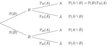
A tree diagram organizes conditional probabilities: each branch carries the probability of the next event given the path so far.

The probability of a leaf (a complete path) is the product of the probabilities along its branches (multiplication rule).
The probability of an event is the sum of the probabilities of the leaves realizing it (total probability).
Probabilities on branches leaving one node add up to $1$ .

A two-level tree: multiply along a path, add over the leaves. For instance (A) is the sum of the first and third leaf probabilities. — A two-level tree: multiply along a path, add over the leaves. For instance $\P(A)$ is the sum of the first and third leaf probabilities.

Theorem 32.5 (Bayes’ formula)

Let $B_1, \dots, B_n$ be a partition of $\Omega$ as above and $A$ an event with $\P(A) > 0$ . Then

\pcond{A}{B_j} = \frac{\P(B_j)\,\pcond{B_j}{A}}{\sum_{i=1}^{n} \P(B_i)\,\pcond{B_i}{A}} .

Proof. $\pcond{A}{B_j} = \frac{\P(A \cap B_j)}{\P(A)}$ ; expand the numerator by the multiplication rule and the denominator by total probability. ∎

Example 32.6 (Screening test)

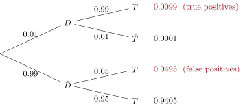
A disease affects $1\%$ of a population. A test detects it with probability $0.99$ (sensitivity) and gives a false positive with probability $0.05$ . Given a positive test, the probability of actually having the disease is

\frac{0.01 \times 0.99}{0.01\times0.99 + 0.99\times0.05} = \frac{0.0099}{0.0099 + 0.0495} = \frac{1}{6} \approx 0.17 .

Despite the accurate test, five positives out of six are false — because the disease is rare. Confusing $\pcond{A}{B}$ with $\pcond{B}{A}$ is the prosecutor’s fallacy.

The screening test as a tree (D: diseased, T: positive test). The two positive leaves (red) have total weight 0.0594, of which the false positives contribute five sixths. — The screening test as a tree ( $D$ : diseased, $T$ : positive test). The two positive leaves (red) have total weight $0.0594$ , of which the false positives contribute five sixths.

32.3 Independence

Definition 32.7 (Independent events)

Two events $A$ and $B$ are independent if

\P(A \cap B) = \P(A)\,\P(B) .

When $\P(B) > 0$ , this is equivalent to $\pcond{B}{A} = \P(A)$ : knowing $B$ does not change the probability of $A$ .

Proposition 32.8

If $A$ and $B$ are independent, so are $A$ and $\bar B$ (and $\bar A$ and $\bar B$ ).

Proof. $\P(A \cap \bar B) = \P(A) - \P(A \cap B) = \P(A) - \P(A)\P(B) = \P(A)\bigl(1 - \P(B)\bigr) = \P(A)\,\P(\bar B)$ . ∎

Remark 32.9

Do not confuse independent ( $\P(A\cap B) = \P(A)\P(B)$ ) with incompatible ( $A \cap B = \varnothing$ ). Two incompatible events of nonzero probability are never independent: knowing one occurred guarantees the other did not.

Definition 32.10 (Independent repetitions)

When an experiment is repeated $n$ times so that the outcome of each trial does not influence the others, the probability of a specified sequence of outcomes is the product of the individual probabilities. This is the model underlying the binomial distribution (Chapter 33).

32.4 Exercises

Exercise 32.1 ★

A card is drawn from a standard 52-card deck. Compute the probability that it is a king, given that it is a face card (jack, queen or king). Are the events “king” and “heart” independent?

Solution

Solution of Exercise 32.1.

There are $12$ face cards, of which $4$ are kings: $\pcond{\text{face}}{\text{king}} = \frac{4}{12} = \frac13$ .

Independence: $\P(\text{king} \cap \text{heart}) = \frac{1}{52}$ (the king of hearts), and $\P(\text{king})\,\P(\text{heart}) = \frac{4}{52}\times\frac{13}{52} = \frac{1}{52}$ . Equal: the events are independent.

Exercise 32.2 ★

An urn contains 5 red and 3 blue balls. Two balls are drawn in succession without replacement.

Draw the probability tree.
Compute the probability that both are red, and the probability that the second is red.

Solution

Solution of Exercise 32.2.

1. First branch: red $\frac58$ , blue $\frac38$ ; second branches (without replacement): after red, red $\frac47$ / blue $\frac37$ ; after blue, red $\frac57$ / blue $\frac27$ .

2. $\P(RR) = \frac58 \times \frac47 = \frac{5}{14}$ . By total probability,

\P(\text{2nd red}) = \frac58\cdot\frac47 + \frac38\cdot\frac57 = \frac{20 + 15}{56} = \frac58 .

(The same as the first draw — by symmetry, the second ball is a uniformly random ball of the urn.)

Exercise 32.3 ★

Two fair dice are rolled. Let $A$ = “the sum is $7$ ”, $B$ = “the first die shows $3$ ”, $C$ = “the sum is $6$ ”. Determine whether $A$ and $B$ are independent, then whether $B$ and $C$ are.

Solution

Solution of Exercise 32.3.

$\P(A) = \frac{6}{36} = \frac16$ (six pairs sum to $7$ ), $\P(B) = \frac16$ , and $A \cap B = \{(3,4)\}$ has probability $\frac{1}{36} = \P(A)\P(B)$ : $A$ and $B$ are independent. (The sum $7$ is special: whatever the first die, exactly one value of the second gives it.)

$\P(C) = \frac{5}{36}$ and $B \cap C = \{(3,3)\}$ : $\P(B \cap C) = \frac{1}{36} \neq \frac16 \times \frac{5}{36} = \frac{5}{216}$ . Not independent.

Exercise 32.4 ★★

A factory has three machines producing respectively $50\%$ , $30\%$ and $20\%$ of total output, with defect rates $1\%$ , $2\%$ and $4\%$ .

What proportion of the production is defective?
A randomly chosen item is defective. What is the probability it came from the third machine?

Solution

Solution of Exercise 32.4.

1. Total probability with the partition by machine:

\P(D) = 0.5\times0.01 + 0.3\times0.02 + 0.2\times0.04 = 0.005 + 0.006 + 0.008 = 0.019 = 1.9\% .

2. Bayes: $\pcond{D}{M_3} = \dfrac{0.008}{0.019} = \dfrac{8}{19} \approx 0.42$ . The machine producing only a fifth of the output accounts for over $40\%$ of the defects.

Exercise 32.5 ★★

In Example 32.6, at what disease prevalence $p$ (instead of $1\%$ ) would a positive test mean at least a $90\%$ chance of disease? Solve the inequality and comment.

Solution

Solution of Exercise 32.5.

The condition is

\frac{0.99\,p}{0.99\,p + 0.05\,(1-p)} \geq 0.9 .

The denominator is positive, so this reads $0.99p \geq 0.891p + 0.045 - 0.045p$ , i.e. $0.144\,p \geq 0.045$ , i.e.

p \geq \frac{0.045}{0.144} = 0.3125 .

The test alone reaches $90\%$ certainty only if the disease already affects more than $31\%$ of the tested population — which is why mass screening of rare diseases requires confirmation tests.

Exercise 32.6 ★★

A biased coin lands heads with probability $p \in \intoo{0}{1}$ . It is tossed three times, tosses being independent.

Compute the probability of the event $E$ = “exactly two heads”.
For which $p$ is $\P(E)$ maximal?

Solution

Solution of Exercise 32.6.

1. Three sequences realize $E$ (HHT, HTH, THH), each of probability $p^2(1-p)$ by independence: $\P(E) = 3p^2(1 - p)$ .

2. $f(p) = 3p^2 - 3p^3$ has $f'(p) = 6p - 9p^2 = 3p(2 - 3p)$ , positive then negative on $\intoo{0}{1}$ : maximum at $p = \frac23$ , where $\P(E) = 3\cdot\frac49\cdot\frac13 = \frac49$ .

Exercise 32.7 ★★★

(Monty Hall.) A prize hides behind one of three doors. You pick a door; the host, who knows where the prize is, opens one of the two remaining doors, always revealing an empty one (choosing at random if both are empty), and offers you to switch to the other closed door. Using Bayes’ formula, compute the probability of winning if you switch, and if you do not.

Solution

Solution of Exercise 32.7.

Say you picked door 1 and the host opened door 3 (event $H_3$ ). With $B_i$ = “prize behind door $i$ ”, $\P(B_i) = \frac13$ and

\pcond{B_1}{H_3} = \frac12, \qquad \pcond{B_2}{H_3} = 1, \qquad \pcond{B_3}{H_3} = 0

(if the prize is behind your door, the host chooses between doors 2 and 3 at random; if it is behind door 2, he is forced to open 3). Bayes:

\pcond{H_3}{B_1} = \frac{\frac13\cdot\frac12}{\frac13\cdot\frac12 + \frac13\cdot1 + 0} = \frac{1/6}{1/2} = \frac13, \qquad \pcond{H_3}{B_2} = \frac{\frac13}{\frac12} = \frac23 .

Staying wins with probability $\frac13$ , switching with probability $\frac23$ .

Exercise 32.8 ★★★

An information channel transmits bits. Each bit is flipped by noise with probability $\varepsilon = 0.1$ , independently. To protect a bit, it is sent three times and decoded by majority.

Compute the probability that the decoded bit is wrong.
The received word is $101$ . What is the probability that the sent bit was $1$ ? (Assume $0$ and $1$ are sent with equal probability.)

Solution

Solution of Exercise 32.8.

1. The majority is wrong when at least two of the three copies are flipped:

3\varepsilon^2(1-\varepsilon) + \varepsilon^3 = 3(0.01)(0.9) + 0.001 = 0.028,

much smaller than $\varepsilon = 0.1$ : repetition coding works.

2. If $1$ was sent (as $111$ ), receiving $101$ requires exactly one flip: probability $\varepsilon(1-\varepsilon)^2 = 0.081$ . If $0$ was sent ( $000$ ), two flips are needed: $\varepsilon^2(1-\varepsilon) = 0.009$ . Bayes with equal priors:

\pcond{101}{\,\text{sent }1} = \frac{0.081}{0.081 + 0.009} = 0.9 .

The majority decoding ( $101 \mapsto 1$ ) is indeed the more probable guess.

32.5 Problem: The doctor, the judge and the spam filter

Problem 32.1

Weekend problem — Bayes’ formula against the base-rate fallacy: why a $99\,\%$ test can mean $2\,\%$ , why a one-in-a-million match convicts nobody, and how your mailbox thinks

A test that catches $99\,\%$ of cases comes back positive — and the true probability of disease is below $2\,\%$ . A DNA profile matching one person in a million is found — and the suspect is probably innocent. Both statements are correct, both have been misjudged by doctors and courts, and both are settled by one line of this chapter: Bayes’ formula (Theorem 32.5). This problem trains it on urns, then in the clinic, the courtroom and the inbox.

Part I — Fluency.

A fair coin chooses urn I ( $2$ red, $1$ blue) or urn II ( $1$ red, $3$ blue), then one ball is drawn. Compute $\P(\text{red})$ with the law of total probability (Theorem 32.3).
The ball is red: compute $\P(\text{urn I} \mid \text{red})$ .
One die roll: are the events “even” and “ $\leq 4$ ” independent (Definition 32.7)? And “even” and “ $\leq 3$ ”?
Two independent smoke alarms each trigger with probability $0.9$ in a fire. Using Proposition 32.8, compute the probability that at least one triggers.
Two cards without replacement: compute $\P(\text{two kings})$ with the multiplication rule (Proposition 32.2).

Part II — The doctor. A disease affects $1$ person in $1\,000$ . The test detects $99\,\%$ of the sick (sensitivity) but also fires on $5\,\%$ of the healthy (false positives).

Natural frequencies: imagine $100\,000$ people. How many are sick, how many healthy? How many positives does each group produce, and how many positives in all?
From the counts, compute $\P(\text{sick} \mid \text{positive})$ . Absorb the shock.
Recompute it with Bayes’ formula and check the agreement.
In surveys, most physicians answer “about $99\,\%$ ”. Name the two conditional probabilities being confused, and explain why the tiny base rate drives the true answer.
A second, independent test also comes back positive. Update: taking $1.9\,\%$ as the new prior, compute $\P(\text{sick} \mid \text{two positives})$ . What is evidence accumulation doing?
Compute $\P(\text{sick} \mid \text{positive})$ if the same test is used only on a high-risk group with prevalence $5\,\%$ . Deduce the public-health moral about mass screening of rare conditions.

Part III — The judge.

A crime-scene DNA profile matches one person in a million. The suspect, found by searching a database of the city’s $10$ million inhabitants, matches. Expected number of innocent matches in the city? Given only the match, what is $\P(\text{innocent} \mid \text{match})$ , roughly?
Name the fallacy — which probability did the prosecutor quote, which one did the court need? — and its exact parallel with question 9.
The independence trap: two rare tragedies in one family were once squared into “one in $73$ million” by treating them as independent, convicting an innocent mother (the Sally Clark case). If the events share family risk factors so that the second, given the first, is $5$ times likelier than the base rate, recompute the order of magnitude — and state the lesson about multiplying probabilities.
The defense can cheat too: “ten innocents match, so the match proves nothing” ignores everything else. What does Bayes’ formula do with several pieces of evidence, and what single sentence should every juror know?

Part IV — The spam filter.

Your mail is $40\,\%$ spam. The word “lottery” appears in $15\,\%$ of spam and $0.5\,\%$ of honest mail. A message contains it: compute $\P(\text{spam} \mid \text{lottery})$ .
Error-correcting repetition (Exercise 32.8 continued): with flip probability $\varepsilon = 0.1$ , majority decoding of five copies fails with what probability? Compare with the three-copy code.
A bit crosses $4$ independent noisy relays, each flipping it with probability $0.1$ : it arrives correct exactly when the number of flips is even. Compute that probability twice: by summing the binomial terms, and by the elegant formula $\frac{1 + (1 - 2\varepsilon)^4}{2}$ .
Real spam filters multiply the evidence of many words as if independent (“naive” Bayes). Why is that assumption false for words like “win” and “lottery” — and why does the filter work well anyway? (One or two sentences.)
Finale — Bayes as the arithmetic of belief: prior $\times$ likelihood, renormalize, posterior. Replay the three verdicts (clinic, courtroom, inbox) in one sentence each, then list the three traps this problem exposed: forgotten base rates, fake independence, and evidence read one piece at a time.

Solution

Solution of Problem 32.1.

1. $\P(\text{red}) = \frac12 \cdot \frac23 + \frac12 \cdot \frac14 = \frac13 + \frac18 = \frac{11}{24}$ .

2. $\P(\text{I} \mid \text{red}) = \dfrac{\frac12 \cdot \frac23}{\frac{11}{24}} = \dfrac{1/3}{11/24} = \dfrac{8}{11}$ .

3. $\P(\text{even} \cap \leq 4) = \P(\{2, 4\}) = \frac13$ and $\P(\text{even})\P(\leq 4) = \frac12 \cdot \frac23 = \frac13$ : independent (unexpectedly!). For $\leq 3$ : $\P(\{2\}) = \frac16$ against $\frac12 \cdot \frac12 = \frac14$ : dependent.

4. The complements of independent events are themselves independent, so

\P(\text{none}) = 0.1 \times 0.1 = 0.01, \qquad \P(\text{at least one}) = 0.99 .

5. $\frac{4}{52} \times \frac{3}{51} = \frac{1}{221}$ .

6. Sick: $100$ ; healthy: $99\,900$ . Positives: $99$ true (99 % of $100$ ) and $4\,995$ false (5 % of $99\,900$ ): $5\,094$ positives in all.

7. $\P(\text{sick} \mid +) = \frac{99}{5\,094} \approx 1.9\,\%$ : of the people the test flags, fewer than one in fifty is actually sick.

8. $\dfrac{0.001 \times 0.99}{0.001 \times 0.99 + 0.999 \times 0.05} = \dfrac{0.00099}{0.05094} \approx 0.019$ : the counts and the formula agree.

9. Confused: $\P(+ \mid \text{sick}) = 99\,\%$ (the test’s advertised quality) with $\P(\text{sick} \mid +)$ (the patient’s actual question). With a base rate of $\frac{1}{1000}$ , the sick are so rare that even a $5\,\%$ leak from the huge healthy majority swamps the true positives fifty to one.

10. $\dfrac{0.019 \times 0.99}{0.019 \times 0.99 + 0.981 \times 0.05} \approx 28\,\%$ . Each independent positive multiplies the odds by the same factor: evidence accumulates, and a third positive would push past $90\,\%$ — which is why confirmatory tests exist.

11. $\dfrac{0.05 \times 0.99}{0.05 \times 0.99 + 0.95 \times 0.05} \approx 51\,\%$ : on a high-risk group the same test is informative. Moral: screen where the base rate is substantial; mass-screening a rare condition manufactures false alarms by the thousand.

12. Expected innocent matches: $10^7 \times 10^{-6} = 10$ . Among the roughly $11$ matching people ( $10$ innocent, $1$ guilty — if the culprit is in the city), the suspect found by the match alone is innocent with probability about $\frac{10}{11} \approx 91\,\%$ .

13. The prosecutor quoted $\P(\text{match} \mid \text{innocent}) = 10^{-6}$ ; the court needed $\P(\text{innocent} \mid \text{match})$ — question 9’s confusion under oath. (And in the real case that popularized these errors, a second blunder compounded it: see question 14.)

14. Naive squaring: $\left(\frac{1}{8500}\right)^2 \approx \frac{1}{72 \text{ million}}$ . With the second tragedy five times likelier given the first: $\frac{1}{8500} \times \frac{5}{8500} \approx \frac{1}{14.5 \text{ million}}$ — five times larger, and still ignoring that the alternative hypothesis must be weighed by Bayes too. Lesson: multiplying probabilities requires independence, and shared causes (genetics, environment) destroy it.

15. Bayes multiplies the likelihood ratios of all the evidence into one posterior: the match, the alibi, the fibers, each shifting the odds. The juror’s sentence: ask how probable the evidence is under both hypotheses, and never mistake the one conditional for its reverse.

16. $\dfrac{0.4 \times 0.15}{0.4 \times 0.15 + 0.6 \times 0.005} = \dfrac{0.060}{0.063} \approx 95\,\%$ spam: one word nearly settles it.

17. Five copies fail when $3$ , $4$ or $5$ flip: $\binom53 \varepsilon^3(1-\varepsilon)^2 + \binom54 \varepsilon^4 (1 - \varepsilon) + \varepsilon^5 \approx 0.0086$ — against $0.028$ for three copies: repetition buys reliability at the price of bandwidth.

18. Even flips: $\binom40 0.9^4 + \binom42 0.9^2 0.1^2 + \binom44 0.1^4 = 0.6561 + 0.0486 + 0.0001 = 0.7048$ ; and $\frac{1 + 0.8^4}{2} = \frac{1 + 0.4096}{2} = 0.7048$ : the trick formula tracks the bias $(1 - 2\varepsilon)$ through each relay.

19. Spammy words travel in packs — a message with “lottery” very likely contains “win”, so their joint evidence is weaker than the product pretends. The filter still works because the exaggeration usually pushes in the right direction: classification needs the correct side of $50\,\%$ , not the correct posterior.

20. Clinic: a rare condition turns a strong test into a weak verdict — update from the base rate, then accumulate. Courtroom: a rare match in a large city indicts the city, not the man — likelihoods are not verdicts. Inbox: many weak clues, multiplied, sort the mail — even naively. The three traps: forget the prior and be fooled; fake independence and be very fooled; read evidence piecemeal and never know what you know.