University Mathematics — Year 2 · Bachelor Year 2

21Probability on Countable Spaces

The final three chapters develop the probability theory of the modern MP* program: probability measures on countable sample spaces, discrete random variables, and generating functions. The finite theory of the High School volume acquires its full infrastructure: $\sigma$ -additivity replaces finite additivity, and the summable-family machinery of Chapter 7 is exactly what makes infinite sample spaces workable. The centerpiece results here are the continuity of probability along monotone sequences of events and the Borel–Cantelli lemma.

21.1 Probability spaces

Definition 21.1 (Countable probability space)

Let $\Omega$ be a nonempty finite or countable set (the sample space). A probability measure on $\Omega$ is a map $\P$ from the set $\mathcal{P}(\Omega)$ of all subsets of $\Omega$ (events) to $[0, 1]$ such that:

$\P(\Omega) = 1$ ;
( $\sigma$ -additivity) for every sequence $(A_n)_{n\in\N}$ of pairwise disjoint events,

$\P\Bigl(\,\bigcup_{n \in \N} A_n\Bigr) = \sum_{n=0}^{\infty} \P(A_n) .$

The pair $(\Omega, \P)$ is a (countable) probability space.

Remark 21.2

On a countable $\Omega$ we may take all subsets as events; on uncountable spaces (as needed for continuous models in Year 3) this is no longer possible, and one restricts $\P$ to a suitable collection of events, a $\sigma$ -algebra. All the formulas of this chapter survive that generalization verbatim.

Proposition 21.3 (Elementary rules)

For events $A, B$ and a probability measure $\P$ : $\P(\emptyset) = 0$ ; $\P$ is finitely additive; $\P(A^c) = 1 - \P(A)$ ; if $A \subseteq B$ then $\P(A) \leq \P(B)$ ; and

\P(A \cup B) = \P(A) + \P(B) - \P(A \cap B) .

Proof. Applying $\sigma$ -additivity to $A_0 = \Omega$ , $A_n = \emptyset$ ( $n \geq 1$ ) gives $1 = 1 + \sum_{n\geq1}\P(\emptyset)$ , so $\P(\emptyset) = 0$ ; padding a finite disjoint union with empty sets then gives finite additivity. The rest follows as in the finite case (High School volume): $1 = \P(A) + \P(A^c)$ from $\Omega = A \sqcup A^c$ ; $\P(B) = \P(A) + \P(B \setminus A) \geq \P(A)$ when $A \subseteq B$ ; and decomposing into three disjoint pieces,

\begin{align*} \P(A \cup B) &= \P(A \setminus B) + \P(B \setminus A) + \P(A \cap B)\\ &= \bigl(\P(A) - \P(A\cap B)\bigr) + \bigl(\P(B) - \P(A\cap B)\bigr) + \P(A \cap B), \end{align*}

which is inclusion–exclusion; the general $n$ -set version is Exercise 21.4. ∎

Proposition 21.4 (Distributions on a countable space)

Giving a probability measure on a countable $\Omega = \{\omega_0, \omega_1, \dots\}$ amounts exactly to giving weights $p_i = \P(\{\omega_i\}) \geq 0$ with $\sum_i p_i = 1$ ; then for every $A \subseteq \Omega$ ,

\P(A) = \sum_{\omega \in A} \P(\{\omega\}) ,

an (absolutely convergent) sub-sum of the family $(p_i)$ .

Proof. Given $\P$ , the singletons $\{\omega\}$ , $\omega \in A$ , form a countable disjoint cover of $A$ , so $\sigma$ -additivity forces

\P(A) = \sum_{\omega\in A}\P(\{\omega\}),

an unconditional sub-sum of the nonnegative summable family $(p_i)$ — reordering is harmless precisely because the terms are nonnegative (Chapter 7); in particular $\sum_ip_i = \P(\Omega) = 1$ . Conversely, given nonnegative weights of total sum $1$ , define $\P(A) = \sum_{\omega \in A}p_\omega$ : the family is summable, and $\sigma$ -additivity is exactly the theorem on summation by packets of Chapter 7 applied to the partition of $\bigcup A_n$ into the $A_n$ . ∎

Example 21.5 (Geometric model: waiting for the first head)

Toss a coin with head probability $p \in \intoo{0}{1}$ repeatedly, and let $\Omega = \N^* \cup \{\infty\}$ record the rank of the first head. The natural weights are

\P(\{k\}) = (1 - p)^{k-1}p \quad (k \in \N^*), \qquad \P(\{\infty\}) = 0 ,

a probability measure since $\sum_{k\geq1}(1-p)^{k-1}p = \frac{p}{1 - (1-p)} = 1$ : with probability $1$ the game ends — but the sample space must still contain the possibility that it does not. Countable additivity is what lets us assert $\P(\text{the game ends}) = \sum_k \P(\{k\})$ .

Theorem 21.6 (Monotone continuity)

Let $(A_n)$ be a sequence of events.

If $A_n \subseteq A_{n+1}$ for all $n$ (increasing), then $\P\bigl(\bigcup_n A_n\bigr) = \lim_{n\to\infty} \P(A_n)$ .
If $A_n \supseteq A_{n+1}$ for all $n$ (decreasing), then $\P\bigl(\bigcap_n A_n\bigr) = \lim_{n\to\infty} \P(A_n)$ .

Proof. 1. Disjointify: let $B_0 = A_0$ and $B_n = A_n \setminus A_{n-1}$ . The $B_n$ are pairwise disjoint with $\bigcup_{k \leq n} B_k = A_n$ and $\bigcup_n B_n = \bigcup_n A_n$ . By $\sigma$ -additivity and finite additivity,

\P\Bigl(\bigcup_n A_n\Bigr) = \sum_{n=0}^\infty \P(B_n) = \lim_{N\to\infty}\sum_{n=0}^N \P(B_n) = \lim_{N\to\infty}\P(A_N) .

2. Pass to complements: $(A_n^c)$ is increasing with union $\bigl(\bigcap A_n\bigr)^c$ , and apply part 1: $1 - \P(\bigcap A_n) = \lim (1 - \P(A_n))$ . ∎

Corollary 21.7 (Countable subadditivity)

For any sequence of events, $\P\bigl(\bigcup_n A_n\bigr) \leq \sum_{n=0}^\infty \P(A_n)$ .

Proof. Finite subadditivity $\P(A_0 \cup \dots \cup A_N) \leq \sum_0^N \P(A_n)$ follows from inclusion–exclusion by induction (or from additivity over the disjointified $B_n \subseteq A_n$ ). Let $N \to \infty$ : the left side converges to $\P(\bigcup_n A_n)$ by monotone continuity applied to the increasing sequence $C_N = A_0 \cup \dots \cup A_N$ . ∎

Example 21.8 (The union bound: crude but indestructible)

Subadditivity with finitely many events — the union bound — trades precision for universality. For the birthday problem with $23$ people, bounding the collision probability by the sum over pairs gives

\P(\text{collision}) \leq \binom{23}2\cdot\frac1{365} = \frac{253}{365} \approx 0.693 ,

against the true $0.507$ : off by a wide margin, because collisions overlap. Yet the bound needs no independence, no joint law, nothing but the pair probabilities — which is why, in the weekend problem and throughout Chapter 22, the union bound is the first tool drawn: when it happens to be small, the matter is settled with no further modelling.

Example 21.9 (A six comes, eventually)

Roll a fair die forever and let $B_n = {}$ “at least one six among the first $n$ rolls”, an increasing sequence of events with $\P(B_n) = 1 - (5/6)^n$ . Monotone continuity gives

\P(\text{a six eventually appears}) = \P\Bigl(\bigcup_nB_n\Bigr) = \lim_n\bigl(1 - (5/6)^n\bigr) = 1 .

The point is not the (obvious) limit but the logical step: “eventually” is an event about infinitely many rolls, outside the reach of finite additivity, and monotone continuity — that is, $\sigma$ -additivity — is precisely the axiom that assigns it a probability. Every almost-sure statement in the rest of this book passes through this same narrow door.

21.2 Conditioning and independence

Definition 21.10 (Conditional probability)

For events $A, B$ with $\P(B) > 0$ , the conditional probability of $A$ given $B$ is

\P(A \mid B) = \frac{\P(A \cap B)}{\P(B)} .

The map $A \mapsto \P(A \mid B)$ is itself a probability measure on $\Omega$ .

Remark 21.11

That $A \mapsto \pcond BA$ is again a probability measure is worth a moment: $\pcond B\Omega = 1$ and $\sigma$ -additivity pass through the quotient because intersection with $B$ respects disjoint unions. The practical consequence: every identity of this chapter — inclusion–exclusion, monotone continuity, Borel–Cantelli — may be applied after conditioning, with no new proofs. Probabilists constantly “work under $\pcond B{\cdot}$ ” for exactly this reason.

Example 21.12 (Conditioning can create uniformity)

Roll two fair dice and condition on the sum being $7$ : for each $k \in \intint16$ ,

\pcond{\{S = 7\}}{X = k} = \frac{\P(X = k,\ Y = 7 - k)}{\P(S = 7)} = \frac{1/36}{6/36} = \frac16 :

given a sum of $7$ , the first die is exactly uniform — $7$ is the only total compatible with every face, so the conditioning erases all information about $X$ . Any other total skews the law (given $S = 4$ , the first die is uniform on $\{1, 2, 3\}$ only). Computing a conditional law means renormalizing the joint weights along the conditioning event, nothing more.

Example 21.13 (The second draw is as good as the first)

An urn holds $3$ white and $2$ black balls; draw two without replacement. Everyone agrees $\P(W_1) = \frac35$ ; what is $\P(W_2)$ ? Total probability along the first draw:

\P(W_2) = \pcond{W_1}{W_2}\,\P(W_1) + \pcond{B_1}{W_2}\,\P(B_1) = \frac24\cdot\frac35 + \frac34\cdot\frac25 = \frac{12}{20} = \frac35 :

exactly $\P(W_1)$ . No computation was needed: by symmetry, every ball is equally likely to be the second one drawn, so the second draw — unconditionally — has the same law as the first. Conditioning on the first result changes the odds; not knowing it does not. This exchangeability argument returns in the next chapter for sampling without replacement, where it gives the hypergeometric mean $np$ with no binomial identities at all.

Theorem 21.14 (Compound probabilities, total probability, Bayes)

(Chain rule) If $\P(A_1 \cap \dots \cap A_{n-1}) > 0$ ,

$\P(A_1 \cap \dots \cap A_n) = \P(A_1)\,\P(A_2 \mid A_1)\cdots \P(A_n \mid A_1 \cap \dots \cap A_{n-1}) .$
(Total probability) If $(B_i)_{i \in I}$ is a finite or countable partition of $\Omega$ with $\P(B_i) > 0$ , then for every event $A$ :

$\P(A) = \sum_{i \in I} \P(A \mid B_i)\,\P(B_i) .$
(Bayes) Under the same hypotheses, if moreover $\P(A) > 0$ :

$\P(B_j \mid A) = \frac{\P(A \mid B_j)\,\P(B_j)} {\sum_{i \in I} \P(A \mid B_i)\,\P(B_i)} .$

Proof. 1. Write each conditional probability as a quotient: the right side is

\P(A_1)\cdot\frac{\P(A_1 \cap A_2)}{\P(A_1)}\cdot \frac{\P(A_1 \cap A_2 \cap A_3)}{\P(A_1 \cap A_2)}\cdots \frac{\P(A_1 \cap \dots \cap A_n)}{\P(A_1 \cap \dots \cap A_{n-1})},

a telescoping product: every denominator cancels the preceding numerator, leaving $\P(A_1 \cap \dots \cap A_n)$ . All denominators are $\geq \P(A_1 \cap \dots \cap A_{n-1}) > 0$ by monotonicity, so nothing vanishes. (The hypothesis guards exactly this: conditioning on an event of probability zero is undefined.) 2. The sets $A \cap B_i$ are pairwise disjoint with union $A$ ; apply ( $\sigma$ -)additivity and the definition of conditioning. 3. Both sides of $\P(B_j \mid A)\P(A) = \P(A \mid B_j)\P(B_j)$ equal $\P(A \cap B_j)$ ; divide by $\P(A)$ and expand $\P(A)$ by total probability. ∎

Example 21.15 (The birthday collision, by the chain rule)

With $n$ people whose birthdays are independent and uniform over $365$ days, let $D_n = {}$ “all $n$ birthdays differ”. Conditioning person by person (chain rule):

\P(D_n) = \prod_{k=1}^{n-1}\Bigl(1 - \frac{k}{365}\Bigr),

each new person having to avoid the $k$ days already taken. For $n = 23$ : $\P(D_{23}) \approx 0.493$ — a shared birthday is already more likely than not. The heuristic that explains the smallness of $23$ : taking logarithms, $-\ln \P(D_n) \approx \sum_{k<n}\frac k{365} = \frac{\binom n2}{365}$ , and $\binom{23}2 = 253$ gives $253/365 \approx 0.693 \approx \ln 2$ . What matters is the number of pairs, which grows quadratically: collision problems live on the scale $n \sim \sqrt{365}$ , not $n \sim 365$ — the birthday paradox is a square root in disguise.

Example 21.16 (Monty Hall, by Bayes)

A prize hides behind one of three doors, uniformly. You pick door $1$ ; the host, who knows where the prize is, opens one of the other doors, always empty (choosing uniformly when he has a choice), say door $3$ . Let $B_i = {}$ “prize behind door $i$ ” and $A = {}$ “host opens door $3$ ”. Then $\pcond{B_1}{A} = \frac12$ , $\pcond{B_2}{A} = 1$ , $\pcond{B_3}{A} = 0$ , so by Bayes (Theorem 21.14),

\P(B_2 \mid A) = \frac{1\cdot\frac13} {\frac12\cdot\frac13 + 1\cdot\frac13 + 0\cdot\frac13} = \frac23 :

switching doors wins two times out of three. The computation locates the popular confusion exactly: the host’s move is informative (he could not open door $2$ if the prize were there), and Bayes’ formula is the bookkeeping device that converts this asymmetry into the $\frac23$ . Conditioning on “what was seen” rather than on “what is true” is the whole art of the formula.

Example 21.17 (The Chevalier de Méré’s two bets)

Two seventeenth-century wagers, settled by independence. Bet one: at least one six in $4$ rolls of a die,

\P = 1 - \Bigl(\frac56\Bigr)^{\!4} \approx 0.518 > \frac12 .

Bet two: at least one double-six in $24$ rolls of two dice,

\P = 1 - \Bigl(\frac{35}{36}\Bigr)^{\!24} \approx 0.491 < \frac12 .

De Méré reasoned that $24$ rolls at chance $\frac1{36}$ should match $4$ rolls at chance $\frac16$ (same ratio $\frac{24}{36} = \frac46$ ); the failure of this proportionality — probabilities of unions do not scale linearly — is said to have prompted his letter to Pascal, and thereby the birth of probability theory. The correct comparison is through logarithms: $n$ trials at chance $p$ succeed at least once with probability $1 - (1-p)^n \approx 1 - \eu^{-np}$ , so the honest invariant is $np$ : here $4\cdot\frac16 = \frac23$ versus $24\cdot\frac1{36} = \frac23$ — equal! The two bets differ only at the second order in $p$ , and by just enough to move one across the fifty-percent line: small probabilities are a domain where intuition needs the exponential, not the ruler.

Remark 21.18 (Common fallacies of conditioning)

Three recurrent confusions, all visible in the examples above. (i) Inversion: $\pcond BA$ and $\pcond AB$ differ by the factor $\P(A)/\P(B)$ — a test that is $99\%$ accurate on the sick may still leave a positive patient almost certainly healthy when the disease is rare (Exercise 21.3); quoting $\pcond{\text{sick}}{ \text{positive}}$ where $\pcond{\text{positive}}{ \text{sick}}$ is meant is the base-rate fallacy. (ii) Conditioning on the wrong event: in Monty Hall, the correct conditioning event is “the host opened door $3$ ”, not “the prize is not behind door $3$ ”; the two carry different information, and the whole $\frac23$ hangs on the difference. (iii) Disjoint versus independent: disjoint events of positive probability are never independent ( $\P(A\cap B) = 0 \neq \P(A)\P(B)$ ) — independence is compatibility of information, not absence of overlap.

Definition 21.19 (Independence)

Events $A$ and $B$ are independent if $\P(A \cap B) = \P(A)\P(B)$ . A family $(A_i)_{i \in I}$ of events is (mutually) independent if for every finite subset $J \subseteq I$ ,

\P\Bigl(\bigcap_{i \in J} A_i\Bigr) = \prod_{i \in J} \P(A_i) .

Remark 21.20

Mutual independence is strictly stronger than pairwise independence: with two fair coin tosses, the events “first is a head”, “second is a head”, “both agree” are pairwise independent (each pair has intersection probability $\frac14 = \frac12\cdot\frac12$ ), yet the triple intersection has probability $\frac14 \neq \frac18$ . Note also that if $A, B$ are independent, so are $A, B^c$ (compute: $\P(A \cap B^c) = \P(A) - \P(A\cap B) = \P(A)(1 - \P(B))$ ), hence also $A^c, B^c$ .

Example 21.21 (Independence read off a product structure)

Roll two fair dice: $\Omega = \intint16^2$ with uniform weights. Let $A = {}$ “first die even” and $B = {}$ “second die at least $5$ ”. Counting: $\abs A = 3\cdot6 = 18$ , $\abs B = 6\cdot2 = 12$ , $\abs{A\cap B} = 3\cdot2 = 6$ , so

\P(A\cap B) = \frac6{36} = \frac{18}{36}\cdot\frac{12}{36} = \P(A)\,\P(B) :

independent, and the mechanism is visible — $A$ constrains only the first coordinate, $B$ only the second, and the uniform measure on a product set makes coordinate counts multiply. Every claim of the type “events depending on disjoint groups of tosses are independent” (used massively in the weekend problem) is this computation, wearing more indices.

Example 21.22 (First-step analysis)

For the geometric model of Example 21.5, what is the probability $u$ that the first head falls at an even rank? Condition on toss one: with probability $p$ the rank is $1$ (odd); with probability $q = 1 - p$ the game restarts with all parities flipped, so

u = p\cdot0 + q\,(1 - u) \qquad\Longrightarrow\qquad u = \frac{q}{1 + q} .

One line, no series — and it agrees with the direct summation of Exercise 21.9, which gives $1 - u = \frac1{1+q}$ . This “first-step” technique (condition on the first experiment, recognize a shifted copy of the problem) is the probabilistic form of a recursion, and it is the engine behind the game-duration equations of Exercise 21.6 and the first-passage computations of the weekend problem.

21.3 The Borel–Cantelli lemma

Definition 21.23 (Limit superior of events)

For a sequence $(A_n)$ of events, the event

\limsup_n A_n = \bigcap_{N=0}^{\infty}\ \bigcup_{n \geq N} A_n = \{\omega \in \Omega : \omega \in A_n \text{ for infinitely many } n\}

is the event “ $A_n$ occurs infinitely often”.

Example 21.24 (Translating “infinitely often” and “eventually”)

The complement of $\limsup_nA_n$ is, by de Morgan,

\Bigl(\bigcap_N\bigcup_{n\geq N}A_n\Bigr)^{\!c} = \bigcup_N\bigcap_{n\geq N}A_n^c = \{\omega : \omega \notin A_n \text{ for all large }n\},

the event “eventually, $A_n$ fails” (written $\liminf_nA_n^c$ ). So “ $A_n$ infinitely often” and “ $A_n^c$ eventually” are complementary — keeping this dictionary straight prevents most quantifier accidents. Sample translations for coin tossing: “infinitely many heads” is $\limsup\{X_n = H\}$ ; “only finitely many runs of $100$ heads” is the complement of a limsup; “the running frequency converges to $\frac12$ ” is $\bigcap_j\bigcup_N\bigcap_{n\geq N}\{\abs{\widehat p_n - \tfrac12} < \tfrac1j\}$ — countable operations throughout, so all of these are honest events.

Theorem 21.25 (Borel–Cantelli)

If $\sum_{n} \P(A_n) < \infty$ , then $\P\bigl(\limsup_n A_n\bigr) = 0$ .
If the events $A_n$ are independent and $\sum_n \P(A_n) = \infty$ , then $\P\bigl(\limsup_n A_n\bigr) = 1$ .

Proof. 1. Let $C_N = \bigcup_{n \geq N}A_n$ ; the sequence $(C_N)$ is decreasing with intersection $\limsup A_n$ , and by countable subadditivity (Corollary 21.7)

\P(C_N) \leq \sum_{n \geq N}\P(A_n) \xrightarrow[N\to\infty]{} 0

(tail of a convergent series). Monotone continuity (Theorem 21.6) concludes: $\P(\limsup A_n) = \lim_N \P(C_N) = 0$ .

2. It suffices to show $\P\bigl(\bigcup_{n\geq N}A_n\bigr) = 1$ for every $N$ : indeed, if events $B_N$ all have probability $1$ , then

\P\Bigl(\Bigl(\bigcap_NB_N\Bigr)^{\!c}\Bigr) = \P\Bigl(\bigcup_NB_N^c\Bigr) \leq \sum_N\P(B_N^c) = 0

by countable subadditivity (Corollary 21.7), so the countable intersection $\limsup A_n = \bigcap_N\bigcup_{n\geq N}A_n$ still has probability $1$ . Fix $N$ , and consider for $M > N$ the complement:

\P\Bigl(\bigcap_{n=N}^{M} A_n^c\Bigr) = \prod_{n=N}^{M}\bigl(1 - \P(A_n)\bigr) \leq \prod_{n=N}^{M} e^{-\P(A_n)} = \exp\Bigl(-\sum_{n=N}^M \P(A_n)\Bigr) ,

using independence of the complements and the convexity bound $1 - x \leq e^{-x}$ . As $M \to \infty$ the exponent tends to $-\infty$ by divergence of the series, so by monotone continuity (decreasing sequence) $\P\bigl(\bigcap_{n \geq N}A_n^c\bigr) = 0$ , i.e. $\P\bigl(\bigcup_{n \geq N}A_n\bigr) = 1$ . ∎

Example 21.26 (Infinite runs of heads)

Toss a fair coin forever, and let $A_n$ be the event “tosses $n, n+1, \dots, n + k - 1$ are all heads” (a run of $k$ heads starting at time $n$ ), for fixed $k$ . The events $A_{jk}$ ( $j = 1, 2, \dots$ ), depending on disjoint blocks of tosses, are independent, each of probability $2^{-k}$ , and $\sum_j 2^{-k} = \infty$ : by Borel–Cantelli 2, with probability $1$ infinitely many blocks are all-heads — every fixed pattern recurs infinitely often, almost surely. Conversely, if we let the run length grow, $B_n = {}$ “a run of $2\log_2 n$ heads starts at $n$ ” has $\P(B_n) = n^{-2}$ summable, so almost surely only finitely many such long runs start: Borel–Cantelli calibrates precisely how long the longest runs are.

Example 21.27 (The infinite monkey, quantified)

A monkey types independent uniform letters from a $26$ -letter alphabet. Cut the typescript into disjoint blocks of four letters; the events $A_j = {}$ “block $j$ spells MATH” are independent with $\P(A_j) = 26^{-4}$ , and $\sum_j\P(A_j) = \infty$ : by Borel–Cantelli 2 the monkey types MATH infinitely often, almost surely — and the same holds for any fixed text of any length, blocks adjusted. The quantitative footnote deflates the miracle: $26^4 = 456\,976$ , so the first MATH takes about half a million keystrokes on average, and a Shakespeare play of $10^5$ characters waits of order $26^{10^5}$ blocks — almost sure is a statement about the horizon $\infty$ , not about any horizon a monkey will meet. Borel–Cantelli certifies the limit; the summands’ size tells the story at human scales.

Remark 21.28

In Example 21.26 the underlying sample space (infinite sequences of tosses) is uncountable, so strictly speaking the example lives in the measure-theoretic framework of Year 3; the computations, though, use only the rules proved in this chapter, applied to events determined by finitely many tosses and their countable combinations. This is the standard MP* convention: the theory is stated on countable spaces, and infinite-game examples are treated with the same toolkit.

Remark 21.29 (Perspectives within this volume)

This chapter’s machinery is consumed wholesale by the next two. Indicators turn events into random variables, and $\sigma$ -additivity becomes the summability that defines expectation (Chapter 22); Borel–Cantelli plus a summable tail bound is exactly how the strong law of large numbers for coins is proved there. In Chapter 23, monotone continuity reappears at the decisive moment: the extinction probability of a branching process is defined as the monotone limit $\lim\P(Z_n = 0)$ , and the fixed-point equation it satisfies is obtained by passing to the limit in that increasing sequence — the final theorem of the book stands on this chapter’s first theorem.

Remark 21.30 (Method: three ways to probability one)

Almost-sure statements are proved with three levers, in increasing order of strength. Monotone continuity: exhibit the event as an increasing union (or decreasing intersection) of finite-horizon events with computable probabilities (Example 21.9). Null unions: a countable union of probability-zero events is null (countable subadditivity), so it suffices to kill each bad event separately — this is how “for every $j$ , eventually $\abs{\widehat p_n - p} < 1/j$ ” assembles into convergence. Borel–Cantelli: when the event is a limsup, sum the probabilities; convergence kills it (no independence needed), and divergence plus independence certifies it. Choosing the right lever is usually the whole proof; the weekend problem runs all three in a single argument.

Remark 21.31 (Where this is used)

Monotone continuity and Borel–Cantelli are the two levers of every “almost sure” statement: they drive the recurrence of the random walk in this chapter’s weekend problem, the almost-sure side of the law of large numbers (Chapter 22), and the extinction analysis of branching processes (Chapter 23). The Year 3 volume rebuilds the theory on $\sigma$ -algebras and Lebesgue integration, where the uncountable sample spaces used informally here become fully rigorous.

21.4 Exercises

Exercise 21.1 ★

An urn contains $n$ numbered balls. Balls are drawn one by one without replacement. Compute the probability that ball number $1$ is drawn before ball number $2$ . Generalize: the probability that ball $1$ is drawn first among balls $1, \dots, k$ .

Solution

Solution of Exercise 21.1.

By symmetry: the drawing order induces a uniformly random relative order on balls $1$ and $2$ , so $\P(1 \text{ before } 2) = \frac12$ . Formally: exchanging the positions of balls $1$ and $2$ in a drawing sequence is a bijection of the (equiprobable) outcomes that swaps the event with its complement. Among balls $1, \dots, k$ : the relative order of these $k$ balls is uniform among the $k!$ orderings, and ball $1$ is first in $(k-1)!$ of them: probability $\frac{(k-1)!}{k!} = \frac1k$ .

Exercise 21.2 ★

Show that on $\Omega = \N^*$ the weights $p_k = \frac{1}{k(k+1)}$ define a probability measure, and compute $\P(2\N^*)$ (even outcomes) as a series; show that it equals $1 - \ln 2$ . (Telescope $\frac{1}{2j(2j+1)} = \frac{1}{2j} - \frac{1}{2j+1}$ and use the alternating harmonic series, Chapter 7.)

Solution

Solution of Exercise 21.2.

$\frac{1}{k(k+1)} = \frac1k - \frac1{k+1}$ , so $\sum_{k\geq1} p_k$ telescopes to $1$ : a probability measure. Even outcomes:

\P(2\N^*) = \sum_{j=1}^{\infty}\frac{1}{2j(2j+1)} = \sum_{j=1}^{\infty}\Bigl(\frac{1}{2j} - \frac{1}{2j+1}\Bigr) = \frac12 - \frac13 + \frac14 - \frac15 + \cdots

This is the alternating harmonic series with its first term removed and signs flipped: since $\ln 2 = 1 - \frac12 + \frac13 - \frac14 + \cdots$ (Chapter 7),

\P(2\N^*) = -\bigl(\ln 2 - 1\bigr) = 1 - \ln 2 \approx 0.307 .

Exercise 21.3 ★

(False positives) A disease affects one person in $10\,000$ . A test detects it with probability $0.99$ on the sick, and gives a false positive with probability $0.01$ on the healthy. Compute the probability of being sick given a positive test, and comment.

Solution

Solution of Exercise 21.3.

Let $S$ = sick, $+$ = positive test. Bayes (Theorem 21.14) with the partition $\{S, S^c\}$ :

\P(S \mid +) = \frac{0.99 \times 10^{-4}} {0.99 \times 10^{-4} + 0.01 \times 0.9999} = \frac{0.000099}{0.000099 + 0.009999} \approx 0.0098 ,

below $1\%$ . Although the test is “99% accurate”, a positive result leaves you about $99\%$ likely to be healthy: the false positives among the vast healthy majority swamp the true positives from the tiny sick minority. Screening tests for rare conditions must always be read through this base-rate computation.

Exercise 21.4 ★★

Let $A_1, \dots, A_n$ be events. Prove the inclusion–exclusion formula

\P\Bigl(\bigcup_{i=1}^n A_i\Bigr) = \sum_{\emptyset \neq J \subseteq \{1,\dots,n\}} (-1)^{\abs J + 1}\,\P\Bigl(\bigcap_{i \in J}A_i\Bigr)

by integrating the identity $1 - \prod_{i=1}^n(1 - \mathbf{1}_{A_i}) = \mathbf{1}_{\bigcup A_i}$ over $\Omega$ (i.e. summing weighted by $\P(\{\omega\})$ ).

Solution

Solution of Exercise 21.4.

Pointwise on $\Omega$ : $\omega \in \bigcup A_i$ iff some factor $1 - \mathbf{1}_{A_i}(\omega)$ vanishes, so

\mathbf{1}_{\bigcup A_i} = 1 - \prod_{i=1}^n\bigl(1 - \mathbf{1}_{A_i}\bigr) = \sum_{\emptyset \neq J \subseteq \{1,\dots,n\}} (-1)^{\abs J + 1}\prod_{i \in J}\mathbf{1}_{A_i} ,

expanding the product and moving the $1$ across. Now $\prod_{i\in J}\mathbf{1}_{A_i} = \mathbf{1}_{\bigcap_{i \in J} A_i}$ , and summing against the weights $\P(\{\omega\})$ — legitimate: finitely many bounded terms, each family summable — turns each indicator into the probability of its event, giving the formula.

Exercise 21.5 ★★

(Matching problem, via inclusion–exclusion) $n$ letters are put uniformly at random into $n$ envelopes, one each. Using Exercise 21.4, show that the probability of no correct match is $\sum_{k=0}^n \frac{(-1)^k}{k!} \to e^{-1}$ , and deduce the probability of exactly one match.

Solution

Solution of Exercise 21.5.

Let $A_i$ = “letter $i$ is in the right envelope”. For $J$ of size $k$ , $\P\bigl(\bigcap_{i\in J}A_i\bigr) = \frac{(n-k)!}{n!}$ (fix $k$ letters, permute the rest). By inclusion–exclusion,

\P\Bigl(\bigcup A_i\Bigr) = \sum_{k=1}^n (-1)^{k+1}\binom nk \frac{(n-k)!}{n!} = \sum_{k=1}^n \frac{(-1)^{k+1}}{k!} ,

\P(\text{no match}) = 1 - \P\Bigl(\bigcup A_i\Bigr) = \sum_{k=0}^{n}\frac{(-1)^k}{k!} \xrightarrow[n\to\infty]{} e^{-1} \approx 0.368 .

Exactly one match: a permutation with exactly one fixed point is determined by the choice of the fixed letter ( $n$ ways) and a derangement (no-match arrangement) of the other $n - 1$ ; writing $D_{n-1} = (n-1)!\sum_{k=0}^{n-1}\frac{(-1)^k}{k!}$ for the number of derangements (the first part, scaled by $(n-1)!$ ),

\P(\text{exactly one match}) = \frac{n\,D_{n-1}}{n!} = \frac{D_{n-1}}{(n-1)!} = \sum_{k=0}^{n-1}\frac{(-1)^k}{k!} \xrightarrow[n\to\infty]{} e^{-1} :

in the limit, “no match” and “exactly one match” are equally likely, each with probability $e^{-1}$ .

Exercise 21.6 ★★

A biased coin (head probability $p \in \intoo{0}{1}$ ) is tossed until two consecutive heads appear. Let $q_n$ be the probability that the game lasts more than $n$ tosses. Show, conditioning on the first toss(es), that $q_n = (1-p)\,q_{n-1} + p(1-p)\,q_{n-2}$ for $n \geq 2$ , and deduce that the game ends with probability $1$ . (Show $q_n \to 0$ by comparing with a geometric sequence: both roots of the characteristic equation lie in $\intoo{0}{1}$ in absolute value.)

Solution

Solution of Exercise 21.6.

Condition on the start (chain rule / Theorem 21.14):

first toss T (probability $1 - p$ ): the game restarts afresh; lasting more than $n$ means lasting more than $n - 1$ from there: contribution $(1-p)\,q_{n-1}$ ;
first tosses HT (probability $p(1-p)$ ): restart after two tosses: contribution $p(1-p)\,q_{n-2}$ ;
first tosses HH: the game has ended (within $n$ tosses, $n \geq 2$ ): contributes $0$ .

Hence $q_n = (1-p)q_{n-1} + p(1-p)q_{n-2}$ . The characteristic equation $r^2 = (1-p)r + p(1-p)$ has roots

r_\pm = \frac{(1-p) \pm \sqrt{(1-p)^2 + 4p(1-p)}}{2},

with $\abs{r_\pm} < 1$ : indeed the polynomial $\chi(r) = r^2 - (1-p)r - p(1-p)$ satisfies $\chi(1) = 1 - (1-p) - p(1-p) = p^2 > 0$ and $\chi(-1) = 1 + (1-p) - p(1-p) > 0$ , while $\chi(0) = -p(1-p) < 0$ : one root in $\intoo{-1}{0}$ , one in $\intoo{0}{1}$ . So $q_n = \alpha r_+^n + \beta r_-^n \to 0$ . The events “game lasts more than $n$ ” decrease to “game never ends”; monotone continuity (Theorem 21.6) gives $\P(\text{never ends}) = \lim q_n = 0$ : the game ends almost surely.

Exercise 21.7 ★★★

(Records) Draw an infinite sequence of independent uniform rankings, in the following combinatorial sense: for each $n$ , the relative order of the first $n$ draws is uniform among the $n!$ possibilities, and $R_n = {}$ “the $n$ -th draw is a record (larger than all previous ones)”. Admitting that the events $R_n$ are independent with $\P(R_n) = 1/n$ (prove at least this last equality by symmetry), show using Borel–Cantelli that infinitely many records occur almost surely, but that records at consecutive times $n, n+1$ occur infinitely often with probability — compute $\sum_n \P(R_n \cap R_{n+1})$ and conclude what Borel–Cantelli 1 gives.

Solution

Solution of Exercise 21.7.

$\P(R_n) = 1/n$ : among the first $n$ draws, each of the $n$ relative positions of the last draw is equally likely (uniformity of the relative order), and $R_n$ is the event that it is the largest: probability $1/n$ .

Infinitely many records: $\sum_n \P(R_n) = \sum 1/n = \infty$ and the $R_n$ are independent (admitted), so Borel–Cantelli 2 (Theorem 21.25) gives $\P(\limsup R_n) = 1$ : records never stop, almost surely — but they thin out logarithmically.

Consecutive records: by independence,

\sum_n \P(R_n \cap R_{n+1}) = \sum_n \frac{1}{n(n+1)} < \infty ,

so Borel–Cantelli 1 applies: almost surely, only finitely many times is a record immediately followed by another record. The two halves of the lemma work in tandem: infinitely many records, but (a.s.) eventually never two in a row.

Exercise 21.8 ★★★

(Kochen–Stone flavour, easier version) Let $(A_n)$ be independent events with $\P(A_n) = \frac{1}{n+1}$ . Show that $\P(\limsup A_n) = 1$ , although $\P(A_n) \to 0$ : “individually rare, collectively certain”. Conversely, exhibit a sequence of (dependent) events with $\sum\P(A_n) = \infty$ and $\P(\limsup A_n) = 0$ , showing independence cannot be dropped in Borel–Cantelli 2.

Solution

Solution of Exercise 21.8.

First part: $\sum \P(A_n) = \sum\frac{1}{n+1} = \infty$ with independence: Borel–Cantelli 2 gives $\P(\limsup A_n) = 1$ . Each individual $A_n$ is increasingly unlikely, yet almost every $\omega$ belongs to infinitely many of them.

Counterexample without independence: take $\Omega = \N^*$ with the weights $p_k = \frac{1}{k(k+1)}$ of Exercise 21.2, and $A_n = \{k \in \N^* : k \geq n\}$ . Then

\P(A_n) = \sum_{k \geq n}\Bigl(\frac1k - \frac1{k+1}\Bigr) = \frac1n , \qquad \sum_n \P(A_n) = \infty ,

but the $A_n$ are decreasing, so $\limsup_n A_n = \bigcap_n A_n = \emptyset$ : $\P(\limsup A_n) = 0$ . Divergence of $\sum\P(A_n)$ alone guarantees nothing when the events pile up on a shrinking part of the space — independence is what forbids that conspiracy.

Exercise 21.9 ★

A coin with head probability $p \in \intoo01$ is tossed until the first head. Compute the probability that this happens at an odd rank, and evaluate it for a fair coin.

Solution

Solution of Exercise 21.9.

With $q = 1 - p$ , the first head falls at rank $2j + 1$ with probability $q^{2j}p$ , so

\P(\text{odd rank}) = \sum_{j\geq0}q^{2j}p = \frac{p}{1 - q^2} = \frac{1}{1 + q} .

For a fair coin: $\frac1{1 + 1/2} = \frac23$ . (Sanity check: odd ranks should be likelier, since rank $1$ comes first — and indeed $\frac1{1+q} > \frac12$ always.)

Exercise 21.10 ★★

Let $(A_n)_{n\geq1}$ be independent events with $\P(A_n) = p_n < 1$ . Show that

\P\Bigl(\bigcap_{n\geq1}A_n^c\Bigr) = \prod_{n\geq1}(1 - p_n) := \lim_{N\to\infty}\prod_{n=1}^N(1 - p_n),

and that this limit is $> 0$ if and only if $\sum p_n < \infty$ . Reconcile with Borel–Cantelli: when $\sum p_n = \infty$ , not only does some $A_n$ occur almost surely — infinitely many do.

Solution

Solution of Exercise 21.10.

The events $B_N = \bigcap_{n=1}^N A_n^c$ decrease to $\bigcap_nA_n^c$ , and by independence of the complements $\P(B_N) = \prod_{n=1}^N(1 - p_n)$ ; monotone continuity (Theorem 21.6) gives the displayed limit. Taking logarithms, $\prod(1 - p_n) > 0$ iff $\sum-\ln(1 - p_n) < \infty$ . If $\sum p_n < \infty$ then $p_n \to 0$ and $-\ln(1 - p_n) \sim p_n$ : the log-series converges. If $\sum p_n = \infty$ , then $-\ln(1 - p_n) \geq p_n$ forces divergence, so the product is $0$ . This matches Borel–Cantelli 2: for $\sum p_n = \infty$ , not only is $\P(\text{no }A_n\text{ occurs}) = 0$ , but almost surely infinitely many $A_n$ occur.

Exercise 21.11 ★★

(Banach’s matchbox) A smoker keeps one box of $n$ matches in each pocket and reaches into a uniformly random pocket each time. When he first finds a box empty, what is the probability that the other box contains exactly $k$ matches? Show the answer is $\binom{2n-k}{n}2^{-(2n-k)}$ and check that these probabilities sum to $1$ for $n = 1$ .

Solution

Solution of Exercise 21.11.

Say box $A$ is the one first discovered empty, with the other box holding $k$ . This means: among the first $2n - k$ reaches, exactly $n$ went to $A$ and $n - k$ to $B$ (in some order), and reach number $2n - k + 1$ went to $A$ again, finding it empty. The reaches are independent fair choices, so this event has probability $\binom{2n-k}{n}2^{-(2n-k)}\cdot\frac12$ ; doubling (the empty box can be either one) gives

\P(\text{other box has }k) = \binom{2n-k}{n}\,2^{-(2n-k)} .

For $n = 1$ : $k = 1$ gives $\binom11 2^{-1} = \frac12$ and $k = 0$ gives $\binom21 2^{-2} = \frac12$ : total $1$ , as it must be.

Exercise 21.12 ★★★

( $\sigma$ -additivity is a real axiom) (a) Show that there is no probability measure on $(\N, \mathcal P(\N))$ giving all singletons the same weight. (b) For $A \subseteq \N^*$ , let $d(A) = \lim_n\frac{\abs{A\cap\intint1n}}{n}$ when the limit exists (the natural density). Show $d$ is finitely additive on pairs where all three densities exist, gives every singleton density $0$ and $\N^*$ density $1$ — and conclude that $d$ is not $\sigma$ -additive. (c) Exhibit a set with no density. (Alternate blocks $\intint{2^{2k}}{2^{2k+1}-1}$ in and out.)

Solution

Solution of Exercise 21.12.

(a) If $\P(\{n\}) = c$ for all $n$ , $\sigma$ -additivity forces $1 = \sum_nc$ : impossible, whether $c = 0$ (sum $0$ ) or $c > 0$ (sum infinite). There is no uniform probability on $\N$ .

(b) If $A \cap B = \emptyset$ and $d(A)$ , $d(B)$ exist, then $\abs{(A \sqcup B)\cap\intint1n} = \abs{A\cap\intint1n} + \abs{B\cap\intint1n}$ , so $d(A \sqcup B) = d(A) + d(B)$ : finite additivity on such pairs. Each singleton has counting function eventually constant, so density $0$ , while $d(\N^*) = 1$ . Were $d$ $\sigma$ -additive, $\N^* = \bigsqcup_k\{k\}$ would give $1 = \sum_k 0 = 0$ : density is finitely additive but not $\sigma$ -additive — the axiom has content.

(c) Let $A = \bigcup_{k\geq0}\intint{4^k}{2\cdot4^k - 1}$ (blocks from $4^k$ to $2\cdot4^k - 1$ ). At $n = 2\cdot4^K - 1$ the count is $\sum_{k\leq K}4^k \sim \frac43 4^K$ , giving ratio $\to \frac23$ ; at $n = 4^{K+1} - 1$ the count is unchanged, giving ratio $\to \frac13$ . The ratio oscillates between limits $\frac13$ and $\frac23$ : no density.

21.5 Problem: the simple random walk on $\Z$ is recurrent

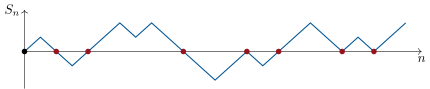
Twenty-four steps of a simple random walk; the red dots mark the returns to the origin. The problem shows that, with probability 1, these dots never stop appearing — yet the waiting time between them has divergent mean. — Twenty-four steps of a simple random walk; the red dots mark the returns to the origin. The problem shows that, with probability $1$ , these dots never stop appearing — yet the waiting time between them has divergent mean.

Problem 21.1

Weekend problem — Pólya’s recurrence theorem on $\Z$ , with the ballot problem and the arcsine flavor on the way

Toss a fair coin forever; let $X_i = \pm1$ be the $i$ -th step and $S_n = X_1 + \dots + X_n$ the simple random walk on $\Z$ , $S_0 = 0$ . As in Example 21.26, all events below are determined by finitely many tosses or are countable combinations of such events, and independence of events depending on disjoint blocks of tosses is part of the model. We write $u_n = \P(S_{2n} = 0)$ and $N_n(k)$ for the number of $\pm1$ -paths of length $n$ from $0$ to $k$ .

Part I — Counting paths.

Show that $N_n(k) = \binom{n}{(n+k)/2}$ when $n + k$ is even and $\abs k \leq n$ , and $0$ otherwise; deduce $\P(S_n = k) = N_n(k)\,2^{-n}$ . Why is every individual path of length $n$ equally likely?
Show $S_{2n+1} \neq 0$ , $u_n = \binom{2n}{n}4^{-n}$ , and compute $u_1, u_2, u_3$ .
Prove $u_n = \frac{2n-1}{2n}\,u_{n-1}$ ; deduce that $(u_n)$ decreases to $0$ , and from Example 6.14 that

$u_n \sim \frac{1}{\sqrt{\pi n}}, \qquad\text{so}\qquad \sum_n u_n = \infty .$
(Reflection principle) For $k \geq 1$ , show that the paths of length $n$ from $1$ to $k$ that touch $0$ are in bijection with the paths from $-1$ to $k$ ; deduce that the number of paths from $0$ to $k$ that stay $> 0$ after time $0$ is $N_{n-1}(k-1) - N_{n-1}(k+1)$ .
(Ballot theorem) Deduce that

$\P\bigl(S_1 > 0, \dots, S_{n-1} > 0 \bigm| S_n = k\bigr) = \frac kn \qquad (k \geq 1) :$

in a count where the winner leads by $k$ out of $n$ ballots, the probability the winner led throughout the count is $k/n$ . Verify by hand for $n = 3$ , $k = 1$ .

Part II — Return to the origin.

Prove the key identity

$\P(S_1 \neq 0,\ S_2 \neq 0,\ \dots,\ S_{2n} \neq 0) = u_n$

(condition on the first step, sum the counts of question 4 over the endpoint, and telescope; finish with $2\binom{2n-1}{n} = \binom{2n}{n}$ ).
Deduce from monotone continuity (Theorem 21.6) that the walk returns to $0$ at least once with probability $1$ , and that $f_n := \P(\text{first return at time }2n)$ satisfies

$f_n = u_{n-1} - u_n = \frac{u_n}{2n-1}, \qquad \sum_{n\geq1}f_n = 1 .$
Show that $\sum_n 2n\,f_n = \infty$ : the return is certain, but the series that would compute the mean waiting time diverges (in the vocabulary of Chapter 22, the return time has infinite expectation).
Prove that for every $k \geq 1$ , $\P(\text{at least } k\text{ returns to }0) = 1$ (decompose over the times of the first $k$ returns: the corresponding toss blocks are disjoint, so the probabilities multiply and sum to $(\sum_nf_n)^k$ ); conclude with monotone continuity:

$\P(S_n = 0 \text{ for infinitely many } n) = 1 :$

the simple random walk on $\Z$ is recurrent.
Show that the walk visits every site $k \in \Z$ almost surely, hence (by recurrence, restarted at the first visit) infinitely often. (The signs of the successive excursions from $0$ are independent fair coins; a positive excursion visits $1$ .)

Part III — Borel–Cantelli and the biased walk.

The events $A_n = \{S_{2n} = 0\}$ satisfy $\sum\P(A_n) = \infty$ ; explain why Borel–Cantelli 2 does not apply to them, and what Borel–Cantelli 1 would give if the series converged. (This is the strategy of the whole Part.)
Now let the coin have bias $p \neq \frac12$ , $q = 1 - p$ . Show $\P(S_{2n} = 0) = \binom{2n}n(pq)^n = u_n\,(4pq)^n$ with $4pq < 1$ , deduce $\sum_n\P(S_{2n} = 0) < \infty$ , and conclude by Borel–Cantelli 1 that the biased walk returns to $0$ only finitely many times, almost surely.
Still for $p \neq \frac12$ : show $\P(S_n = k) \leq \binom{n}{\floor{n/2}}\,(pq)^{n/2}\,(p/q)^{k/2}$ for each fixed $k$ , deduce that every site is visited finitely often almost surely, and conclude $\abs{S_n} \to \infty$ almost surely: the biased walk is transient.
Back to the fair coin: using question 6, compute the probability that $200$ tosses produce no tie ( $S_n \neq 0$ for $1 \leq n \leq 200$ ), numerically $u_{100} \approx 0.056$ . Comment on the slow $1/\sqrt{\pi n}$ decay: ties are certain in the long run but rarer than intuition suggests.
(First passage) Let $T_1$ be the first time the walk hits $1$ . Using the reflection principle for the maximum $M_n = \max_{i\leq n}S_i$ (proved in question 16, which does not depend on this one), or directly from question 7 by conditioning on the first step, show $\P(T_1 = 2n - 1) = f_n$ ; deduce $\P(T_1 < \infty) = 1$ while the mean-time series $\sum(2n-1)f_n$ diverges.

Part IV — Maxima, last zero, long leads.

(Reflection for the maximum) For $k \geq 1$ , prove

$\P(M_n \geq k) = 2\,\P(S_n > k) + \P(S_n = k)$

by reflecting the path after its first visit to level $k$ .
Deduce $\P(M_{2n} \geq 1) = 1 - u_n$ , i.e. $\P(S_i \leq 0 \text{ for all } i \leq 2n) = u_n$ : the probability of never being ahead equals the probability of never being at zero (question 6) — two different events, one probability.
(Last zero) Let $L_{2n} = \max\{k \leq 2n : S_k = 0\}$ (even). Combining question 6 with independence of disjoint toss blocks, show

$\P(L_{2n} = 2k) = u_k\,u_{n-k} \qquad (0 \leq k \leq n),$

and deduce, with no further computation, the binomial identity $\sum_{k=0}^n u_ku_{n-k} = 1$ .
Show that the law of $L_{2n}$ is symmetric ( $\P(L = 2k) = \P(L = 2n - 2k)$ ) and, using $u_j \sim 1/\sqrt{\pi j}$ , that its extremes are its most likely values. Tabulate for $n = 5$ : $\P(L_{10} = 0) = u_5 \approx 0.246$ versus $\P(L_{10} = 4) = u_2u_3 \approx 0.117$ . Interpret: in a long fair game, the last tie tends to be very early or very late — long leads are the rule, not the exception.
Assemble questions 16–19 into a paragraph on the fluctuation picture of the fair walk: the diffusive scale suggested by question 3, the certainty of return against the divergent mean waiting time, and the arcsine-flavored persistence of leads.

Part V — The renewal identity and Pólya’s theorem.

Prove, by partitioning $\{S_{2n} = 0\}$ over the time of the first return, the renewal identity

$u_n = \sum_{k=1}^n f_k\,u_{n-k} \quad (n \geq 1), \qquad\text{hence}\qquad U(x)\bigl(1 - F(x)\bigr) = 1 \quad (0 \leq x < 1),$

where $U(x) = \sum_{n\geq0}u_nx^n$ and $F(x) = \sum_{n\geq1}f_nx^n$ (justify the radii and the product of series with Chapter 11).
Deduce the recurrence dichotomy: letting $x \to 1^-$ (monotone limits of series with nonnegative coefficients),

$\sum_n u_n = \infty \iff \sum_n f_n = 1 ,$

and check it against questions 3, 7 (fair walk) and 12 (biased walk).
(Dimension $2$ ) The simple walk on $\Z^2$ takes steps $(\pm1, 0)$ , $(0, \pm1)$ uniformly. Show that the rotated coordinates $U_n = X_n + Y_n$ and $V_n = X_n - Y_n$ perform independent fair walks on $\Z$ , deduce

$\P\bigl(S^{(2)}_{2n} = (0,0)\bigr) = u_n^2 \sim \frac1{\pi n}, \qquad \sum_n u_n^2 = \infty ,$

and conclude with questions 21–22 (whose proofs transfer verbatim) that the walk on $\Z^2$ is recurrent.
(Dimension $3$ ) For the simple walk on $\Z^3$ , admit the local estimate $\P(S^{(3)}_{2n} = 0) \leq C\,n^{-3/2}$ (proved with the local limit theorem in the Year 3 volume). Deduce from Borel–Cantelli 1 that the walk on $\Z^3$ is transient, and state the full result: Pólya’s theorem — the simple random walk is recurrent in dimensions $1$ and $2$ , transient in dimension $3$ and higher.
Synthesis. List the exact role played by: path counting and reflection; monotone continuity; independence of disjoint toss blocks; Borel–Cantelli 1; the renewal identity. Which single analytic fact ( $u_n \sim 1/\sqrt{\pi n}$ , hence $\sum u_n = \infty$ but $\sum u_n^2 = \infty$ and $\sum n^{-3/2} < \infty$ ) decides between recurrence and transience in each dimension?

Solution

Solution of Problem 21.1.

1. A path of length $n$ is determined by the set of its up-steps; ending at $k$ means $u$ up-steps and $n - u$ down-steps with $u - (n - u) = k$ , i.e. $u = \frac{n+k}2$ : possible iff $n + k$ is even and $\abs k \leq n$ , in $\binom{n}{(n+k)/2}$ ways. Each specific path is one point of the fair product measure on $n$ tosses: probability $2^{-n}$ . Hence $\P(S_n = k) = N_n(k)2^{-n}$ .

2. $S_n$ has the parity of $n$ , so $S_{2n+1} \neq 0$ ; and $u_n = N_{2n}(0)4^{-n} = \binom{2n}n4^{-n}$ . Values: $u_1 = \frac12$ , $u_2 = \frac6{16} = \frac38$ , $u_3 = \frac{20}{64} = \frac5{16}$ .

3. $\dfrac{u_n}{u_{n-1}} = \dfrac{\binom{2n}n}{4\binom{2n-2}{n-1}} = \dfrac{(2n)(2n-1)}{4n^2} = \dfrac{2n-1}{2n} < 1$ : decreasing. By Example 6.14, $\binom{2n}n \sim \frac{4^n}{\sqrt{\pi n}}$ , so $u_n \sim \frac1{\sqrt{\pi n}} \to 0$ , and $\sum u_n$ diverges by comparison with $\sum n^{-1/2}$ .

4. Given a path from $1$ to $k$ touching $0$ , reflect its initial segment (up to the first visit to $0$ ) through the horizontal axis: the result is a path from $-1$ to $k$ , and the operation is an involution — every path from $-1$ to $k \geq 1$ must cross $0$ , and reflecting its initial segment back recovers the original. Hence the touching paths number $N_{n-1}(k + 1)$ (from $-1$ to $k$ the displacement is $k + 1$ ). A path from $0$ to $k$ staying $> 0$ after time $0$ starts with an up-step and then goes from $1$ to $k$ in $n - 1$ steps without touching $0$ : there are $N_{n-1}(k-1) - N_{n-1}(k+1)$ of them.

5. With $m = \frac{n+k}2$ , using $\binom{n-1}{m-1} = \frac mn\binom nm$ and $\binom{n-1}{m} = \frac{n-m}n\binom nm$ :

\frac{N_{n-1}(k-1) - N_{n-1}(k+1)}{N_n(k)} = \frac{\binom{n-1}{m-1} - \binom{n-1}{m}}{\binom nm} = \frac{m - (n - m)}{n} = \frac kn .

For $n = 3$ , $k = 1$ : $N_3(1) = 3$ paths ( $++-$ , $+-+$ , $-++$ ), of which only $++-$ stays positive ( $+-+$ returns to $0$ at time $2$ ): one out of three, and $\frac kn = \frac13$ .

6. By symmetry the probability is $2\P(S_i > 0\ \forall i \leq 2n)$ . Summing over the endpoint $2k$ and using question 4 (with $n$ replaced by $2n$ ):

\P(S_i > 0\ \forall i) = 2^{-2n}\sum_{k\geq1} \bigl(N_{2n-1}(2k-1) - N_{2n-1}(2k+1)\bigr) = 2^{-2n}\,N_{2n-1}(1),

a telescoping sum. Now $N_{2n-1}(1) = \binom{2n-1}{n}$ and $2\binom{2n-1}n = \binom{2n}n$ (Pascal), so the displayed probability is $2\cdot2^{-2n}\binom{2n-1}n = \binom{2n}n4^{-n} = u_n$ .

7. The events $D_n = \{S_i \neq 0,\ i \leq 2n\}$ decrease, with intersection “no return ever”; by monotone continuity and question 6, $\P(\text{no return}) = \lim u_n = 0$ : the walk returns almost surely. Moreover $f_n = \P(D_{n-1}) - \P(D_n) = u_{n-1} - u_n$ , and by question 3

u_{n-1} - u_n = u_n\Bigl(\frac{2n}{2n-1} - 1\Bigr) = \frac{u_n}{2n-1}; \qquad \sum_{n\geq1}f_n = u_0 - \lim u_n = 1 .

8. $2n\,f_n = \frac{2n}{2n-1}u_n \geq u_n$ , and $\sum u_n = \infty$ (question 3): the series $\sum 2nf_n$ diverges. The first return is certain but has no finite mean waiting time — the walk is null recurrent, in the vocabulary that Chapter 22 will provide.

9. The event “at least $k$ returns” is the disjoint countable union, over $0 < n_1 < \dots < n_k$ , of the events “the first $k$ returns happen exactly at times $2n_1, \dots, 2n_k$ ”. Such an event is the intersection of $k$ events depending on the disjoint toss blocks $\intint1{2n_1}$ , $\intint{2n_1+1}{2n_2}$ , …, each block requiring a fresh walk to make its first return after exactly the allotted number of steps; by independence of the blocks its probability is $f_{n_1}f_{n_2-n_1}\cdots f_{n_k-n_{k-1}}$ . Summing by packets (Chapter 7, all terms nonnegative):

\P(\text{at least }k\text{ returns}) = \Bigl(\sum_{n\geq1}f_n\Bigr)^{\!k} = 1^k = 1 .

The events decrease in $k$ , so by monotone continuity $\P(\text{infinitely many returns}) = 1$ : recurrence.

10. By question 9 the walk makes infinitely many excursions away from $0$ . The first step of each excursion is a fresh coin, independent of everything before: the probability that the first $m$ excursions all start downward is $2^{-m}$ . To reach $1$ the walk only needs one upward excursion start (from $<0$ it must pass through $0$ before reaching $1$ , steps being $\pm1$ ), so $\P(\text{never hit }1) \leq 2^{-m}$ for every $m$ : the walk hits $1$ almost surely. Decomposing over the (almost surely finite) hitting time, the walk restarted there is a fresh walk started at $1$ : by induction it hits every $k \geq 1$ almost surely, and by symmetry every $k \leq -1$ . Finally, restarting at the first visit to $k$ , question 9 applies to the fresh walk: every site is visited infinitely often, almost surely.

11. The events $A_n = \{S_{2n} = 0\}$ are far from independent (being at $0$ at time $2n$ makes being at $0$ at time $2n + 2$ far likelier than $u_{n+1}$ ), so Borel–Cantelli 2 is unavailable, and indeed the whole work of Part II was to replace it. The other direction needs no independence: if $\sum\P(A_n)$ converges, Borel–Cantelli 1 yields finitely many returns almost surely. That implication is the engine of every transience proof below.

12. A return at time $2n$ requires $n$ up- and $n$ down-steps: $\P(S_{2n} = 0) = \binom{2n}np^nq^n = u_n(4pq)^n$ , and $4pq = 1 - (p - q)^2 < 1$ for $p \neq \frac12$ . Since $u_n \leq 1$ , the series $\sum\P(S_{2n} = 0)$ is dominated by the geometric $\sum(4pq)^n$ : convergent. By Borel–Cantelli 1, $\P(S_{2n} = 0 \text{ infinitely often}) = 0$ : finitely many returns, almost surely.

13. For $n + k$ even, $\P(S_n = k) = \binom{n}{\frac{n+k}2}p^{\frac{n+k}2}q^{\frac{n-k}2}$ ; the binomial coefficient is at most the central one, and $p^{\frac{n+k}2}q^{\frac{n-k}2} = (pq)^{n/2}(p/q)^{k/2}$ , giving the stated bound $\leq 2^n(pq)^{n/2}(p/q)^{k/2} = (4pq)^{n/2}(p/q)^{k/2}$ , summable in $n$ since $\sqrt{4pq} < 1$ . Borel–Cantelli 1: site $k$ is visited finitely often almost surely; the union over $k \in \Z$ of the exceptional null events is still null (countable subadditivity). Almost surely every site is visited finitely often, so the integer sequence $(S_n)$ leaves every bounded window for good: $\abs{S_n} \to \infty$ .

14. $\P(S_n \neq 0,\ 1 \leq n \leq 200) = u_{100} = \binom{200}{100}4^{-100} \approx \frac1{\sqrt{100\pi}} \approx 0.056$ : more than a one-in-twenty chance that $200$ fair tosses never tie. The decay $1/\sqrt{\pi n}$ is excruciatingly slow: certainty of a tie (question 7) is compatible with very long tie-free stretches — a first taste of the arcsine phenomena of Part IV.

15. Condition on the first step. If $X_1 = +1$ then $T_1 = 1$ , and $f_1 = \frac12$ matches. If $X_1 = -1$ , the walk must climb from $-1$ to $1$ ; by the block decomposition, returning to $0$ for the first time at time $2n$ splits as: one step down, then a fresh walk started at $-1$ first reaching $0$ — equivalently a fresh walk first reaching $+1$ — in $2n - 1$ steps, or the symmetric event upward. Both signs contribute equally:

f_n = 2\cdot\tfrac12\,\P(T_1 = 2n - 1) = \P(T_1 = 2n-1) .

Hence $\P(T_1 < \infty) = \sum f_n = 1$ , while $\sum_n(2n - 1)f_n = \sum_n u_n = \infty$ by question 7: the walk reaches $1$ almost surely, in infinite mean time.

16. Partition $\{M_n \geq k\}$ by the terminal value $S_n = m$ . For $m \geq k$ the condition $M_n \geq k$ is automatic. For $m < k$ , reflect the path after its first visit to level $k$ : this is a bijection between $\{M_n \geq k, S_n = m\}$ and $\{S_n = 2k - m\}$ (every path ending at $2k - m > k$ visits $k$ ; reflecting back is the inverse). Hence

\P(M_n \geq k) = \sum_{m > k}\P(S_n = m) + \P(S_n = k) + \sum_{m < k}\P(S_n = 2k - m) = 2\P(S_n > k) + \P(S_n = k).

17. At even time $2n$ with $k = 1$ : $\P(S_{2n} = 1) = 0$ and $\P(S_{2n} > 1) = \P(S_{2n} \geq 2)$ , so

\P(M_{2n} \geq 1) = 2\P(S_{2n} \geq 2) = \P(S_{2n} \geq 2) + \P(S_{2n} \leq -2) = 1 - u_n .

Thus $\P(S_i \leq 0\ \forall i \leq 2n) = u_n$ : the walk never leads in the first $2n$ steps exactly as often as it never ties (question 6) — two quite different events, carried by the same $u_n$ .

18. $\{L_{2n} = 2k\} = \{S_{2k} = 0\} \cap \{\text{the walk of the tosses } 2k+1, \dots, 2n \text{ has no zero}\}$ . The two events depend on disjoint toss blocks, so they are independent; the first has probability $u_k$ , the second $u_{n-k}$ by question 6 applied to the fresh $(2n-2k)$ -step walk. Hence $\P(L_{2n} = 2k) = u_ku_{n-k}$ . Since $L_{2n}$ takes exactly the values $0, 2, \dots, 2n$ , these probabilities sum to $1$ : $\sum_{k=0}^nu_ku_{n-k} = 1$ , a binomial identity delivered by a probabilistic partition.

19. Symmetry is immediate: $u_ku_{n-k} = u_{n-k}u_k$ . As $u_j$ decreases in $j$ , the product $u_ku_{n-k}$ is smallest for central $k$ and largest at the extremes $k \in \{0, n\}$ , where it equals $u_n$ ; quantitatively $u_ku_{n-k} \approx \frac1{\pi\sqrt{k(n-k)}}$ in the bulk, against $u_n \approx \frac1{\sqrt{\pi n}}$ at the edges. For $n = 5$ : $\P(L_{10} = 0) = \P(L_{10} = 10) = u_5 = \frac{63}{256} \approx 0.246$ , while $\P(L_{10} = 4) = u_2u_3 = \frac38\cdot\frac5{16} = \frac{15}{128} \approx 0.117$ . In a long fair game the last equalization is most likely near the very beginning or the very end: one player typically leads for enormous stretches, with no bias in the coin.

20. The picture: at time $n$ the walk lives at scale $\sqrt n$ (the binomial spread of question 3 — $u_n \sim 1/\sqrt{\pi n}$ is the height of the central peak); it returns to $0$ infinitely often with probability $1$ (Part II), yet the waiting time between returns has divergent mean (question 8), which is why single excursions can occupy a positive fraction of any horizon; correspondingly the last tie of a $2n$ -step game is spread out with extreme values most likely (questions 18–19), and never-leading has the same slowly decaying probability $u_n$ as never-tying (question 17). Certainty in the limit, persistence at every finite horizon: that is the fair walk.

21. Partition $\{S_{2n} = 0\}$ ( $n \geq 1$ ) by the first return time $2k$ , $1 \leq k \leq n$ : the first block of $2k$ tosses realizes a first return, the remaining $2n - 2k$ tosses realize a return of a fresh walk, and the blocks are independent: $u_n = \sum_{k=1}^nf_ku_{n-k}$ . Both series $U(x) = \sum u_nx^n$ , $F(x) = \sum f_nx^n$ have radius $\geq 1$ (coefficients in $\intcc01$ ), and the Cauchy product (Chapter 11) gives, for $0 \leq x < 1$ ,

U(x) - 1 = \sum_{n\geq1}\Bigl(\sum_{k=1}^n f_ku_{n-k}\Bigr)x^n = F(x)\,U(x), \qquad\text{i.e.}\qquad U(x)\bigl(1 - F(x)\bigr) = 1 .

22. As $x \uparrow 1$ , $U(x)$ and $F(x)$ increase (nonnegative coefficients); every partial sum $\sum_{n\leq N}u_n$ is a limit of $\sum_{n\leq N}u_nx^n \leq U(x)$ , so $U(x) \uparrow \sum u_n \in \intoc0{+\infty}$ , and likewise $F(x) \uparrow f = \sum f_n$ . If $\sum u_n = \infty$ : $1 - F(x) = 1/U(x) \to 0$ , so $f = 1$ . If $\sum u_n = S < \infty$ : $1 - f = 1/S > 0$ , so $f < 1$ . Checks: fair walk, $\sum u_n = \infty$ and $f = 1$ (questions 3, 7); biased walk, $\sum u_n(4pq)^n < \infty$ and correspondingly $f = 1 - 1/\sum_{n\geq0}u_n(4pq)^n < 1$ , consistent with the almost-sure finiteness of the number of returns (question 12).

23. For the four steps $(\pm1, 0), (0, \pm1)$ of the $\Z^2$ walk, the increments of $U = X + Y$ and $V = X - Y$ are: $(+,+)$ for $(1,0)$ , $(+,-)$ for $(0,1)$ , $(-,+)$ for $(0,-1)$ , $(-,-)$ for $(-1,0)$ — each pair of signs with probability $\frac14 = \frac12\cdot\frac12$ : the two coordinate walks $(U_n)$ and $(V_n)$ are independent fair walks on $\Z$ . Since $S^{(2)}_{2n} = (0,0)$ iff $U_{2n} = 0$ and $V_{2n} = 0$ ,

\P\bigl(S^{(2)}_{2n} = (0,0)\bigr) = u_n^2 \sim \frac1{\pi n}, \qquad \sum_nu_n^2 = \infty .

The renewal identity of question 21 and the dichotomy of question 22 used nothing one-dimensional (only the decomposition over the first return and disjoint-block independence), so $\sum u_n^{(2)} = \infty$ gives $f^{(2)} = 1$ , and the argument of question 9 upgrades it: the walk on $\Z^2$ returns to the origin infinitely often almost surely.

24. With the admitted bound $\P(S^{(3)}_{2n} = 0) \leq Cn^{-3/2}$ , the series converges, and Borel–Cantelli 1 gives finitely many returns almost surely: the walk on $\Z^3$ is transient (and the same bound with exponent $-d/2$ handles every $d \geq 3$ ). Altogether: Pólya’s theorem — the simple random walk is recurrent on $\Z$ and $\Z^2$ , transient on $\Z^d$ for $d \geq 3$ . A drunk man finds his way home; a drunk bird may not.

25. Path counting and reflection produced the exact laws ( $u_n$ , the ballot theorem, $f_n$ , the maximum, the last zero); monotone continuity converted every limiting statement (“returns at least once”, “infinitely often”) into a limit of finite-horizon probabilities; disjoint-block independence powered the renewal decompositions (questions 9, 18, 21) — it is the countable skeleton of the Markov property; Borel–Cantelli 1 was the transience weapon (questions 12–13, 24), needing no independence; the renewal identity organized everything into the dichotomy $\sum u_n = \infty \iff$ recurrence. The single analytic input is the local estimate $u_n \sim 1/\sqrt{\pi n}$ : its square $1/(\pi n)$ still diverges (dimension $2$ , recurrent), while $n^{-3/2}$ converges (dimension $3$ , transient) — Pólya’s theorem is, in the end, a statement about the divergence of $\sum n^{-d/2}$ .

21.1 Probability spaces

21.2 Conditioning and independence

21.3 The Borel–Cantelli lemma

21.4 Exercises

21.5 Problem: the simple random walk on Z\ZZ is recurrent

21.5 Problem: the simple random walk on $\Z$ is recurrent