Market Making and High-Frequency Trading · Market making
2Fair Value
The same stock quotes on a dozen venues, its index future trades in Chicago and the exchange-traded fund that holds it trades in New Jersey. The market maker’s price is none of these quotes but its own estimate, revised on every message from any of them. In this chapter’s simulated market, where a follower instrument trades on two venues and a leader moves first, the best estimate built from the follower’s own book forecasts its mid five seconds ahead 2.4% better than the mid does. Adding the leader’s price improves the forecast by 3.5% when the leader moves half a second first, and by 12.8% when it moves two seconds first. Small percentages, applied to every quote of every day, are what this chapter is about.
2.1 Mid, weighted mid and microprice
Definition 2.1 (Fair price)
A market maker’s fair price is its estimate, at time , of the efficient price of an instrument from the information it has at : the books of the venues where the instrument trades, the prices of related instruments, and its own recent fills. Quotes are set around it; the gap between a fill’s price and the fair price at the fill is the fill’s expected profit.
The name is chosen against two neighbours. The fair value of a future (One Quant Book 1, chapter 21) is a no-arbitrage price from spot, financing and dividends; the theoretical value of an option (One Quant Book 5, chapter 26) comes from a volatility surface. A fair price can use either as an input, but it is a statistical estimate, revised on every message, and its quality is measured by how well it forecasts.
Three estimators use one venue’s top of book. The mid ignores the queue sizes and . The weighted mid
moves towards the ask when the bid queue is the larger, because a large bid queue is less likely to be exhausted first. The microprice (One Quant Book 7, chapter 8) replaces the fixed formula with a table learned from data: the mid plus the average change of the mid over a horizon, by bucket of the queue imbalance . Stoikov showed that the microprice so estimated forecasts short-term prices better than the mid or the weighted mid.
Example 2.2 (Three estimates of one book)
A book shows 300 shares bid at 99 ticks and 100 offered at 100. The mid is 99.5; the imbalance is 0.75 and the weighted mid 99.75. This chapter’s microprice table, fitted on the first simulated hour with five buckets and a five-second horizon, adds , , , and ticks to the mid for imbalances in , , …, . Here it adds 0.091 and gives 99.59: the data say the weighted mid overstates what the imbalance predicts.
2.2 Fair price across venues
When one instrument trades on several venues, each venue’s book is a noisy, differently delayed view of one efficient price. A venue whose quote has not changed for a second tells less than one that changed a millisecond ago; a venue with a thin book is noisier than the primary market.
Definition 2.3 (Consolidated fair price)
A consolidated fair price is a fair price that combines the books of every venue on which an instrument trades, each weighted by how much its prices tell about the efficient price, in view of its liquidity and of how recently it changed.
A consolidated fair price is not the national best bid and offer (One Quant Book 1, chapter 9), which is a regulatory construct of protected quotes. The market maker cares about information, not protection: a venue that rarely trades may carry a stale best price and deserve almost no weight.
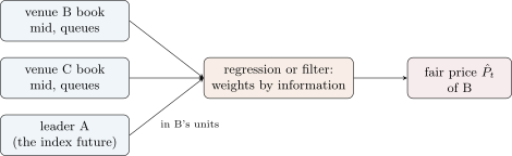
The simplest calibration is a regression: the future mid of the instrument, minus its current mid, on the gaps between each source and the mid. On the chapter’s market (a follower B quoted on two venues, B and C) the weights fitted on the first hour are 0.73 on B’s own microprice and 0.32 on C’s; they sum to about one, as they should for two measurements of one price, and the second venue earns a third of the weight.
2.3 Fair price across instruments
Definition 2.4 (Cross-instrument fair price)
A cross-instrument fair price is a fair price that also uses the prices of related instruments, translated into the instrument’s own units (by a hedge ratio, a conversion ratio, a currency or a fair-value basis), so that a move of a related instrument that leads is reflected before the instrument’s own book shows it.
An exchange-traded fund’s market maker watches the index future; a receipt’s market maker watches the home listing and the currency (chapter 14); an options market maker watches the underlying. The related instrument must be put in the right units first. For the future of an index and a fund on that index, the translation is the fair-value basis of One Quant Book 1, chapter 21; in the chapter’s market the two share one efficient price, so no translation is needed.
With the leader’s mid added to the regression, the weights become 0.74 on B’s microprice, 0.22 on C’s and 0.18 on the leader’s; when the leader moves two seconds before B, the leader’s weight rises to 0.27, B’s own to 0.89, and C’s falls to . The regression is using the lead that chapter 8 will estimate and trade.
2.4 Filtering: the fair price as a state
Regressions weigh sources by their average information. A filter weighs each observation when it arrives, by how long it has been since the last one.
Definition 2.5 (Fair-price filter)
A fair-price filter treats the efficient price as a hidden state, a random walk with variance per second, and every source’s price as an observation of it with noise variance . On an observation from source at time , the previous update having been at , it propagates and updates:
It is the local-level Kalman filter of One Quant Book 4, chapter 19, run on irregular times; a quiet period raises and hence the weight of the next observation, which is exactly the behaviour a stale venue calls for (Listing 2.1).
Proposition 2.6 (Steady state under regular observations)
If one source is observed every seconds, the posterior variance converges to
Proof. A fixed point of satisfies ; its positive root is . The map is increasing and concave with slope below one at the fixed point, so the iteration converges from any positive start. ∎
With square ticks a second, and ten observations a second, and : each new mid moves the fair price by a fifth of its surprise. The chapter’s filter uses , the variance rate of the efficient price over the first hour, and for each source the variance of its gap to the mid five seconds later, 0.104, 0.123 and 0.134 for B, C and the leader.
2.5 Evaluating a fair price
A fair price is judged by what it forecasts. In a simulation the efficient price is known and the error can be measured against it; in a live market only future prices are observed, and the natural target is the mid some seconds later. Both targets are used below, on a grid of 0.1 seconds over the second simulated hour, with every parameter fitted on the first hour.
| RMSE (ticks), lead 0.5 s | change against the mid (%) | |||
| estimator of B’s fair price | efficient price | mid in 5 s | lead 0.5 s | lead 2 s |
| mid | 0.962 | 0.549 | 0.0 | 0.0 |
| weighted mid | 0.963 | 0.542 | ||
| microprice | 0.957 | 0.536 | ||
| consolidated, regression | 0.947 | 0.542 | ||
| consolidated, filter | 0.961 | 0.559 | ||
| cross-instrument, regression | 0.930 | 0.529 | ||
| cross-instrument, filter | 0.941 | 0.544 | ||
The last two columns are changes of the error against the mid five seconds ahead, averaged over three simulated markets. Three lessons stand out. The book of the instrument itself says little: in this market every estimator built from it is within 2.5% of the mid. The leader says more, and more the further ahead it is (Figure 2.2); at a two-second lead the cross-instrument fair price removes an eighth of the error. And the filter, whose variances were set by a rule of thumb, does worse than the regression, which was fitted to the very target it is scored on: calibrate a fair price to what it will be used to forecast.
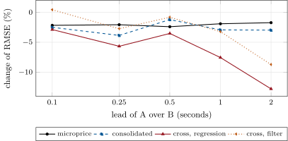
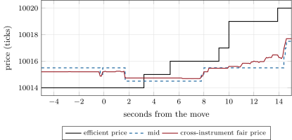
hf_fairvalue.by_lag.Figure 2.3 shows why. After the largest ten-second move of the second hour, B’s efficient price climbs five ticks, its mid follows a tick at a time over several seconds, and the cross-instrument fair price moves ahead of the mid as soon as the leader’s book has moved. In Figure 2.2, with three markets per point, the curves are noisy (the half-second lead happens to show less than the quarter-second one); the trend is not.
hf_fairvalue.window.Remark 2.7 (How good is good)
A 3% lower error sounds like nothing. A market maker earns a fraction of the spread on every fill and loses the adverse selection that its fair price failed to foresee (chapter 1); chapter 6 shows the fills that move against it are concentrated in the moments when its fair price was most wrong. The value of a fair price is measured in adverse selection saved, per fill, times all the fills of a year.
2.6 Tutorial: three markets, seven fair prices
Goal. Build the chapter’s fair prices for a follower instrument quoted on two venues with a leader, fit them on one hour and score them on the next. End state: the table above and Figures 2.2 and 2.3.
- Markets.
hf_fairvalue.markets(lag)simulates A, and B and C whose efficient price is A’slagseconds later, each with its own order flow. The filter.
firm.fairprice.FairFilteris Definition 2.5 in code; its C++20 and Rust twins reproduce the same numbers on a shared fixture of 3 000 observations.class FairFilter: """Local-level Kalman filter over irregular observations from several sources.""" def __init__(self, q: float, r, x0: float | None = None, p0: float = 1e6): self.q, self.r = float(q), [float(v) for v in r] self.x = math.nan if x0 is None else float(x0) self.p, self.t = float(p0), None def update(self, t: float, src: int, y: float) -> float: if self.t is None: self.t = t if math.isnan(self.x): self.x = y self.p = self.r[src] return self.x self.p += self.q * (t - self.t) self.t = t k = self.p / (self.p + self.r[src]) self.x += k * (y - self.x) self.p = (1.0 - k) * self.p return self.x def predict(self, t: float) -> tuple[float, float]: return self.x, self.p + self.q * (t - self.t)Listing 2.1. The fair-price filter: propagate for the elapsed time, then update. code/firm/fairprice/firm_fairprice.py The regressions. The future mid minus the mid on the gaps between each source and the mid, fitted on the first hour.
def _design(lv: dict, kind: str) -> np.ndarray:
    base = lv["mid"]
    cols = {"consolidated": [lv["micro"] - base, lv["c_micro"] - base],
            "cross": [lv["micro"] - base, lv["c_micro"] - base, lv["a_mid"] - base]}[kind]
    return np.column_stack(cols)


@functools.cache
def weights(lag: float = LAG, seed: int = 31) -> dict:
    """Least-squares weights of the regression fair prices, fitted on the first hour: future mid minus mid on the
    gaps between each source and the mid."""
    _, lv, _, fut = _levels(lag, seed, True)
    return {k: np.linalg.lstsq(_design(lv, k), fut - lv["mid"], rcond=None)[0] for k in ("consolidated", "cross")}
Listing 2.2. Regression fair prices: design and weights. code/hft/02-fair-value/python/hf_fairvalue.py - Score.
table(lag)averages the errors over three seeds;fig_fairvalue.pywrites the figures’ data.
What to change next. Make venue C thin and slow and watch its weight fall; let the leader’s lead vary through the day and refit the weights every ten minutes.
2.7 Build: the fair-price engine
Purpose. Streaming fair prices for every Quoter of the book, with a core fast enough for the hot path.
Interface. weighted_mid, imbalance, fit_micro(imb, spread, dmid, n), micro(…, g); FairFilter(q, r).update(t, src, y) -> estimate, predict(t); run_filter; rmse.
Rules. Parameters are fitted on data before the period they are used on. Sources are translated into the instrument’s units before they enter. The first observation initialises the state. The C++20 (cpp/firm_fairprice.hpp) and Rust (rust/) filters perform the same operations in the same order.
Acceptance tests. code/firm/fairprice/tests/: the weighted mid and the microprice by hand; one Kalman step by hand; the fixture reproduced by the Python reference and, in cpp/ and rust/, by the twins, to ticks.
Stretch. Staleness-dependent noise ; a two-state filter with the leader’s lead as a state; online refitting of the weights.
Sources and further reading
- S. Stoikov, “The micro-price: a high-frequency estimator of future prices”, Quantitative Finance 18(12), 2018.
- One Quant Book 4, chapter 19 (the Kalman filter) and One Quant Book 7, chapter 8 (the microprice and the order-book features).
2.8 Exercises
Exercise 2.1 ★
A book shows 300 shares bid at 99 and 100 offered at 100. Compute the weighted mid.
Solution
Solution of Exercise 2.1.
.
Exercise 2.2 ★
With the chapter’s microprice table, what is the microprice of a one-tick book 99/100 whose imbalance is 0.9?
Solution
Solution of Exercise 2.2.
Bucket adds 0.220: .
Exercise 2.3 ★
The filter holds with ; , . A mid of 101 arrives 0.4 seconds after the last update. Give the gain and the new fair price.
Solution
Solution of Exercise 2.3.
, ; .
Exercise 2.4 ★★
Using Proposition 2.6, compute and for , and ten observations a second, and say what happens to when the source slows to one observation a second.
Solution
Solution of Exercise 2.4.
: , . At one observation a second, , and : rarer observations each count for more.
Exercise 2.5 ★★
Why can a filter with variances set by rule of thumb forecast worse than the plain mid, while a regression fitted on the same history does not?
Solution
Solution of Exercise 2.5.
The filter assumes the sources’ errors are independent white noise around the current efficient price. The mids of this market lag the efficient price for seconds, so their errors are autocorrelated and shared; the filter weighs them wrongly and adds its own smoothing lag. The regression learns the weights that best forecast the target it is judged on, whatever the error structure.
Exercise 2.6 ★★
From Figure 2.2, read the improvement of the cross-instrument regression at a one-second lead.
Solution
Solution of Exercise 2.6.
About (the point at a one-second lead reads ).
Exercise 2.7 ★★★
Coding. Compute table(1.0) and give the change of the error of the cross-instrument filter against the mid, five seconds ahead.
Solution
Solution of Exercise 2.7.
for the filter, against for the regression at the same lead.
Exercise 2.8 ★★★
Find the flaw. “Our new microprice table cuts the forecast error by 9% on today’s data, on which we fitted it.”
Solution
Solution of Exercise 2.8.
In-sample: a table fitted on a day always fits that day better than the mid. Fit it on one period and score it on the next, as the chapter does (first hour, second hour), and report the out-of-sample change.
2.9 Problem: Whose Price Is It
Problem 2.1
Weekend problem — whose price is it
An exchange-traded fund trades on two venues and follows its index future. You must give its market maker one number, updated on every message.
Part I — One book.
- Define the fair price and distinguish it from a future’s fair value.
- Write the weighted mid and explain its direction.
- How is a microprice table fitted, and why only on one-tick books?
- Give the chapter’s table and the microprice of a 99/100 book at imbalance 0.75.
- By how much does the microprice improve on the mid as a five-second forecast?
Part II — Many venues, many instruments.
- Define a consolidated fair price and say why it is not the national best bid and offer.
- Give the regression weights on B’s and C’s microprices and interpret their sum.
- Define a cross-instrument fair price and say what must happen to the leader’s price before it enters.
- Give the three weights with the leader at a half-second and at a two-second lead.
Part III — The filter.
- Write the fair-price filter’s propagate and update steps.
- Prove Proposition 2.6.
- Why does a stale source get more weight on its next observation?
- Give the chapter’s and and how each was estimated.
- Why did the filter forecast worse than the regression?
Part IV — The verdict.
- State the named result: the five-second forecast error of the mid, the microprice and the cross-instrument fair price at a half-second lead, and the share of the cross-instrument improvement that the leader brings.
- How does the improvement change with the lead?
- Why are three simulated hours too few to trust the shape of Figure 2.2 point by point?
- What does Figure 2.3 show?
- How is a fair price’s quality turned into money?
- In one sentence: what makes a fair price better than the mid?
Solution
Solution of Problem 2.1.
- An estimate of the efficient price from everything observed, updated on every message; a future’s fair value is a no-arbitrage price from spot, financing and dividends.
- : the larger bid queue is less likely to be exhausted first, so the next move is more likely up.
- Average change of the mid over the horizon by imbalance bucket, on one-tick books, where the imbalance is informative and the mid is well defined.
- ; .
- 2.4% lower error at a half-second lead (0.536 against 0.549 ticks).
- Combines every venue’s book by information; the NBBO is a regulatory construct of protected quotes, blind to staleness and depth.
- 0.73 and 0.32; they sum to about one because both measure one price.
- Uses related instruments’ prices after translating them into the instrument’s units (hedge ratio, conversion, currency, basis).
- 0.74, 0.22, 0.18 at a half-second lead; 0.89, , 0.27 at two seconds.
- , , , .
- See Proposition 2.6.
- Its variance has grown with the time since the last update, so the gain is larger.
- square ticks a second from the first hour’s efficient-price variance; , 0.123, 0.134 from each source’s gap to the mid five seconds later.
- Its noise model (independent white errors) is wrong for mids that lag; the regression is fitted to the target.
- Mid 0.549, microprice 0.536, cross-instrument 0.529 ticks; the leader brings 65% of the improvement over the mid (the consolidated fair price without it is at 0.542).
- It grows with the lead: at half a second, at one, at two.
- Each point averages three hours whose errors are autocorrelated; the differences between neighbouring leads are of the size of the noise.
- The mid follows the efficient price a tick at a time over seconds; the cross-instrument fair price moves as soon as the leader has.
- By the adverse selection it saves per fill, times the fills of a year.
- It uses information the mid does not contain: the queues, other venues, and above all the instruments that move first.
2.10 Interview questions
Interview question 2.1 ★ trader
The bid queue is ten times the ask queue. Where is the fair price, and why?
Solution
Solution of Interview question 2.1.
Close to the ask: the bid queue is far less likely to be exhausted first, so the next mid change is more likely up; how close is an empirical question, answered by a microprice table.
What the interviewer is looking for: direction and that the size of the adjustment must be estimated.
Interview question 2.2 ★★ researcher
How would you evaluate a fair-price model when the efficient price is never observed?
Solution
Solution of Interview question 2.2.
Score it as a forecast of observable future prices (the mid or the next trade some seconds later), out of sample, against the mid as a baseline; check markouts of the fills it would have generated.
What the interviewer is looking for: a forecasting target, out-of-sample evaluation, and a baseline.
Interview question 2.3 ★★ researcher
Derive the steady-state Kalman gain of a random walk observed with noise every seconds.
Solution
Solution of Interview question 2.3.
Fixed point of : , , .
What the interviewer is looking for: the Riccati fixed point done cleanly.
Interview question 2.4 ★★ developer
A fair-price service consumes feeds from eight venues. What must each update carry, and what do you do when one feed goes silent?
Solution
Solution of Interview question 2.4.
Venue, instrument, exchange and receive timestamps, sequence number, prices and sizes. A silent feed’s observations age: its weight must fall (a filter does it through the elapsed time), and a gap in sequence numbers must mark its book invalid until recovered.
What the interviewer is looking for: timestamps, sequence numbers, staleness handling.
Interview question 2.5 ★★ trader
Your fund’s fair price uses the index future. The future’s market closes early today. What changes?
Solution
Solution of Interview question 2.5.
The leader’s source disappears: its weight must go to zero at the close, the quotes widen because the fair price becomes less precise, and the fund is priced from its own books and whatever proxies remain open.
What the interviewer is looking for: source availability, wider quotes when information drops.
Interview question 2.6 ★★★ researcher
Two venues’ mids measure one price with independent noises of variance and . What weights minimise the variance of the combination, and when is ignoring the second venue optimal?
Solution
Solution of Interview question 2.6.
Minimise : , variance . Ignoring the second venue is optimal only if its noise is infinite; with correlated noises the optimal weight can be zero or negative.
What the interviewer is looking for: inverse-variance weights and the correlated case.