3Inventory Models

A market maker who has just bought three times in a row owns stock nobody has asked for yet. Lowering both quotes a little makes the next trade more likely to be a sale; lowering them too much gives the spread away. Avellaneda and Stoikov turned the trade-off into a control problem whose approximate solution fits on one line, and simulated it: at their benchmark risk aversion the inventory-aware quotes earned 5% less than symmetric quotes of the same average width, with half the standard deviation. This chapter solves the problem, reproduces their experiment, solves the variant with a running inventory penalty exactly, and then takes the answer to a large-tick market, where a quote can only be at the touch or absent: there, on this chapter’s simulated sessions, controlling inventory turns a losing quoter into a break-even one.

3.1 The market maker’s control problem

Ho and Stoll set the problem in 1981: a dealer whose prices depend on its inventory because holding inventory is risky. The modern form keeps the ingredients and makes the order flow explicit. The mid is $S_t=S_0+\sigma W_t$ (arithmetic, over a trading session). The market maker quotes a bid $S^b_t=S_t-\delta^b_t$ and an ask $S^a_t=S_t+\delta^a_t$, where the quote depths $\delta^b_t,\delta^a_t$ are its controls (local symbols of this chapter; $\delta$ alone stays the accrual fraction). Market sell orders reach the bid, and market buys the ask, at rates that fall with the depth. Its inventory $q_t$ rises by one on each bid fill and falls by one on each ask fill; its cash $X_t$ moves by the fill prices.

Definition 3.1 (Fill intensity)

The fill intensity of a resting quote is the rate at which it is executed, as a function of its depth $\delta$ from the mid. The inventory models assume $\lambda(\delta)=A\,e^{-k\delta}$, the same on both sides, with $A$ and $k$ constant (local symbols: $A$ is not an annuity and $k$ not a log-moneyness here).

The exponential form is not a law. It comes from assuming that market orders arrive at a constant rate with sizes whose price impact reaches a depth $\delta$ with probability $e^{-k\delta}$; it is convenient because it makes the control problem solvable, and it is testable, since a quoter can measure how often it is filled at each depth (Section 3.5).

3.2 The Avellaneda–Stoikov model

Definition 3.2 (Avellaneda–Stoikov model)

The Avellaneda–Stoikov model is the market maker’s problem with an arithmetic Brownian mid, exponential fill intensities, a horizon $T$ and an exponential utility of terminal wealth: the market maker chooses $\delta^b_t,\delta^a_t$ to maximise $\E\bigl[-\exp\bigl(-\gamma\,(X_T+q_TS_T)\bigr)\bigr]$, with $\gamma>0$ its risk aversion.

The Hamilton–Jacobi–Bellman equation of One Quant Book 4, chapter 9 applies. With the ansatz $u(t,x,s,q)=-\exp(-\gamma(x+\theta(t,s,q)))$, the first-order conditions give the optimal depths as functions of $\theta$’s differences across inventories; Avellaneda and Stoikov then expand $\theta$ to second order in $q$ and obtain the approximate solution below.

3.3 Reservation price and optimal spread

Definition 3.3 (Reservation price)

The reservation price of a market maker holding $q$ is the price at which it is indifferent to its current position and one more or one fewer unit; in the Avellaneda–Stoikov model, approximately

$$S^{\mathrm{res}}_t=S_t-q_t\,\gamma\sigma^2\,(T-t).$$

Proposition 3.4 (The Avellaneda–Stoikov quotes)

To second order in inventory, the optimal quotes are centred on the reservation price, $S^{b,a}_t=S^{\mathrm{res}}_t\mp\tfrac12\Delta_t$, with total width

$$\Delta_t=\delta^a_t+\delta^b_t=\gamma\sigma^2\,(T-t)+\frac{2}{\gamma}\ln\Bigl(1+\frac{\gamma}{k}\Bigr).$$

The derivation is in Avellaneda and Stoikov’s paper; Proposition 3.6 below derives an exact solution of a close relative.

Two effects are separated. The reservation price moves against the inventory in proportion to risk aversion, variance and the time left: a long market maker quotes lower on both sides, selling more readily and buying less. The width has an inventory-risk part, $\gamma\sigma^2(T-t)$, and a monopoly part, $(2/\gamma)\ln(1+\gamma/k)$, which tends to $2/k$ as $\gamma\to0$: with no risk aversion the market maker still quotes a spread, set by how fast fills fall off with depth. The skew of the quotes is the quote skewing of One Quant Book 2, chapter 15, derived from a model instead of a rule of thumb.

Definition 3.5 (Inventory penalty)

An inventory penalty replaces risk aversion in utility by a cost charged on the position while it is held: the market maker maximises $\E\bigl[X_T+q_TS_T-\alpha q_T^2-\phi\int_0^Tq_t^2\,dt\bigr]$, with a running penalty $\phi$ and a terminal one $\alpha$.

The running penalty is a risk charge the desk chooses, not a preference it has. With $\phi=\tfrac12\gamma\sigma^2$ it charges exactly the variance that the position adds per unit of time; a desk can also set it from a value-at-risk budget.

Proposition 3.6 (Exact solution with an inventory penalty)

With inventory confined to $\{-\bar q,\dots,\bar q\}$, write the value function as $x+qs+h(t,q)$ and put $h=\tfrac1k\ln\omega$. Then $\omega(t)=\exp\bigl(M(T-t)\bigr)z$, with $z_q=e^{-\alpha kq^2}$ and $M$ tridiagonal: $M_{q,q}=-\phi kq^2$ and $Ae^{-1}$ next to the diagonal. The optimal depths are

$$\delta^a(t,q)=\frac1k+h(t,q)-h(t,q-1),\qquad \delta^b(t,q)=\frac1k+h(t,q)-h(t,q+1),$$

and the side that would breach the bound is not quoted.

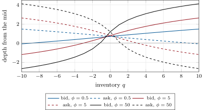
Figure 3.1 shows the solution for the chapter’s parameters. Flat, the market maker quotes symmetric depths above $1/k$; long, it lowers the ask depth and raises the bid depth, and at large inventories the ask depth becomes negative: the model tells the market maker to offer below the mid, which in a real book means crossing the spread. The model has no notion of a spread to cross; chapter 4 bounds the inventory instead.

3.4 The Avellaneda–Stoikov experiment, reproduced

Avellaneda and Stoikov simulated their quotes with $S_0=100$, $T=1$, $\sigma=2$, time steps of 0.005, $k=1.5$ and $A=140$, the mid moving up or down by $\sigma\sqrt{0.005}$ at each step, and compared them with a symmetric strategy that quotes the same average width around the mid. The same experiment, run with firm.invmm on 1 000 paths with the two strategies on common random numbers, gives:

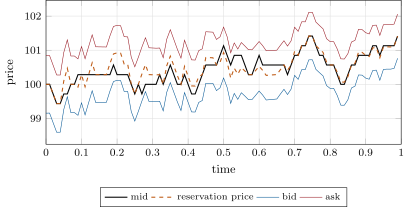
The reproduction agrees with the published tables to within sampling error. Near risk neutrality the two strategies earn the same and the inventory strategy is already less variable; at $\gamma=0.1$ it gives up 5% of the profit for half the standard deviation; at $\gamma=1$ it gives up 27%. Figure 3.2 redraws one path: the quotes follow the reservation price, which leaves the mid whenever inventory builds up.

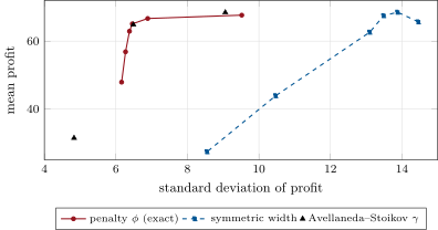
With a running penalty instead of utility, the exact quotes of Proposition 3.6 trace a frontier of mean against standard deviation of profit that lies well above the symmetric quotes’ (Figure 3.3): a small penalty, $\phi=0.5$, keeps 97% of the profit of the best symmetric width (66.7 against 68.5) with half its standard deviation (6.9 against 13.9).

3.5 The limits of the closed forms

Four assumptions carry the model, and each fails somewhere.

Remark 3.7 (What the model leaves out)

(i) Continuous prices. Quotes live on a tick grid; the model’s depths are real numbers. (ii) Exponential intensities. Fills depend on queue position and on the book behind the quote, not on depth alone. (iii) No information. The mid is a martingale unaffected by the fills: there is no adverse selection, so a fill is never bad news (chapter 4 adds it). (iv) Constant parameters. Volatility and order flow vary through the day and with news.

The first two failures are severe in a large-tick market. On Book 7’s simulated stock, an exploring quoter that moved its one-lot quotes at random among the touch and one, two or three ticks behind it, every five seconds for an hour, spent about 1 640 seconds at the touch and got 8 fills, and about 5 280 seconds behind it and got none: the book’s depth behind the touch is never reached by the market orders of this market. The only choice is to rest at the touch or not.

The problem remains a control problem. With $\lambda$ the fill intensity of one lot at the touch per side and $c$ the capture per fill net of adverse selection, the value $h(t,q)$ solves

and the market maker rests on a side exactly when that side’s bracket is positive (Listing 3.2). The quote never moves away from the touch; the skew of the continuous model becomes a decision about which sides to show.

3.6 Tutorial: from the model to a quoter

The penalised quoters trade almost as much and hold a fraction of the inventory; they lose less, and vary far less. With six sessions the means are imprecise (the symmetric quoter’s standard error is $40), and the direction is the lesson rather than the size: in this market a filled quote is followed on average by an adverse move, so the inventory the symmetric quoter accumulates is where it loses.

3.7 Build: the inventory-model library

3.8 Exercises

Exercise 3.1 ★

A market maker with $\gamma=0.1$, $\sigma=2$ and half the session left ($T-t=0.5$) holds 3 units at a mid of 100. Compute its reservation price.

Solution

Solution of Exercise 3.1.

$S^{\mathrm{res}}=100-3\times0.1\times4\times0.5=99.4$.

Exercise 3.2 ★

With $k=1.5$, compute the Avellaneda–Stoikov width at the start of the session ($T-t=1$) for $\gamma=0.1$, and its monopoly part.

Solution

Solution of Exercise 3.2.

$\Delta=0.1\times4\times1+20\ln(1+0.1/1.5)=0.40+1.29=1.69$; the monopoly part is 1.29.

Exercise 3.3 ★

A quote rests at depth 0.5 for 1 000 seconds and is filled 40 times; at depth 1.0 for 1 000 seconds it is filled 18 times. Estimate $A$ and $k$.

Solution

Solution of Exercise 3.3.

$\ln(40/18)=0.5k$ gives $k=1.60$; $A=0.04\,e^{0.5k}=0.0889$ fills a second.

Exercise 3.4 ★★

Show that the Avellaneda–Stoikov width tends to $2/k$ as $\gamma\to0$ at the horizon, and explain why a risk-neutral market maker still quotes a spread.

Solution

Solution of Exercise 3.4.

At the horizon the inventory term vanishes and $(2/\gamma)\ln(1+\gamma/k)\to2/k$ as $\gamma\to0$ (since $\ln(1+x)\sim x$). A risk-neutral market maker still trades off the capture per fill, which grows with depth, against the fill rate, which falls with it: $\delta Ae^{-k\delta}$ is maximised at $\delta=1/k$.

Exercise 3.5 ★★

From Figure 3.1, at which inventory does the ask depth turn negative for $\phi=5$, and what would the quote mean in a real book?

Solution

Solution of Exercise 3.5.

Between $q=3$ (ask depth 0.011) and $q=4$ ($-0.217$). A negative depth offers below the mid: in a real book it crosses the spread, i.e. the market maker sells aggressively to the bid.

Exercise 3.6 ★★

Why does the symmetric strategy earn more on average than the inventory strategy at $\gamma=0.1$, and why is that no reason to prefer it?

Solution

Solution of Exercise 3.6.

The inventory strategy skews: whenever it holds a position, one of its quotes is closer to the mid than half the average width, and that is the side that fills, so it earns less per fill (it fills slightly more often, 97.0 times against 91.7, for less money). What it gains is variance: 6.49 against 14.00. For any positive risk aversion its certainty equivalent is the higher one, and that is what it maximises.

Exercise 3.7 ★★★

Coding. With CJSolution(140, 1.5, 5.0, 1.0, 30, 1.0, 200), give the depths at the start of the session for $q=0$ and for $q=3$.

Solution

Solution of Exercise 3.7.

$q=0$: both depths 0.804. $q=3$: bid 1.550, ask 0.011.

Exercise 3.8 ★★★

Find the flaw. “We fitted $A$ and $k$ on our quotes one and two ticks behind the touch in a one-tick stock and got $k=0$: fills do not depend on depth, so we will quote deeper and earn more.”

Solution

Solution of Exercise 3.8.

Quotes behind the touch of a one-tick stock are almost never filled (the chapter’s exploring quoter got none in 5 280 seconds): the fit is on zeros, and $k$ is not identified. Depth cannot be chosen continuously in a large-tick book; the decision is whether to rest at the touch.

3.9 Problem: Three Buys in a Row

Problem 3.1

Weekend problem — three buys in a row

A market maker has just bought three times. Decide what to quote next, first in the textbook model, then in the market it actually trades.

Part I — The model.

1. State the Avellaneda–Stoikov model: dynamics, controls and objective.
2. Define the fill intensity and give the model’s assumption.
3. Define the reservation price and write its approximate form.
4. Write the approximate width and split it into its two parts.
5. Compute the reservation price and quotes at $q=3$, $\gamma=0.1$, $\sigma=2$, $k=1.5$, $T-t=0.5$, $S=100$.

Part II — The exact solution.

6. Define an inventory penalty and relate the running penalty to risk aversion.
7. Derive the depths of Proposition 3.6 from the Hamilton–Jacobi–Bellman equation.
8. Why does the mid’s volatility drop out of the equation for $h$?
9. Give the depths at $q=0$ and $q=3$ for $\phi=5$, and interpret the negative ask depth at large inventory.

Part III — The experiment.

10. Give the experiment’s parameters.
11. Give profit and standard deviation of both strategies at the three risk aversions, and compare with the paper.
12. At which risk aversion do the two strategies’ profits diverge, and by how much?
13. What does the penalty frontier add?

Part IV — The market it trades.

14. What did the exploring quoter find behind the touch, and why?
15. Write the touch-only equation and its decision rule.
16. How were $\lambda$ and $c$ calibrated, and why on separate sessions?
17. State the named result: the P&L and inventory of the symmetric and the penalised quoters on the simulated market, and, in the model, the profit and standard deviation of the two strategies at $\gamma=0.1$.
18. Why are six sessions enough for the direction and not for the size?
19. Which assumption of the model does the simulated market violate most?
20. In one sentence: what should a market maker do after three buys in a row?

Solution

Solution of Problem 3.1.

1. $S_t=S_0+\sigma W_t$; quotes $S\mp\delta^{b,a}$; fills at $Ae^{-k\delta}$; maximise $\E[-e^{-\gamma(X_T+q_TS_T)}]$.
2. The rate at which a resting quote at depth $\delta$ is executed; $\lambda(\delta)=Ae^{-k\delta}$.
3. The indifference price of one more or one fewer unit; $S^{\mathrm{res}}=S-q\gamma\sigma^2(T-t)$.
4. $\gamma\sigma^2(T-t)$ (inventory risk) plus $(2/\gamma)\ln(1+\gamma/k)$ (monopoly).
5. $S^{\mathrm{res}}=99.40$; width $0.2+1.291=1.491$; bid 98.65, ask 100.15.
6. A cost $\phi\int q^2dt+\alpha q_T^2$ on held inventory; $\phi=\tfrac12\gamma\sigma^2$ charges the variance the position adds.
7. See the proof of Proposition 3.6.
8. The value is linear in $s$ ($x+qs+h$), so the second derivative in $s$ is zero; risk enters only through the penalty.
9. 0.804 on both sides at $q=0$; bid 1.550 and ask 0.011 at $q=3$; beyond $q=3$ the ask is below the mid, a crossing order.
10. $S_0=100$, $T=1$, $\sigma=2$, steps 0.005, $k=1.5$, $A=140$, binomial mid, 1 000 paths.
11. $\gamma=0.01$: 68.45 (9.06) against 68.50 (13.91); $\gamma=0.1$: 64.83 (6.49) against 68.15 (14.00); $\gamma=1$: 31.44 (4.83) against 43.30 (10.34); the paper: 68.6 (8.7)/68.8 (12.8), 65.0 (6.6)/68.4 (12.7), 31.4 (5.0)/44.0 (11.0).
12. From $\gamma\approx0.1$: 5% less profit at 0.1, 27% less at 1; at 0.01 they are equal.
13. The exact penalised quotes dominate symmetric widths: $\phi=0.5$ gives 66.7 with sd 6.9 against 68.5 with sd 13.9.
14. Eight fills in 1 640 seconds at the touch and none in 5 280 seconds behind it: market orders here never walk past the touch.
15. $\partial_th-\phi q^2+\lambda\max(0,c+h(q-1)-h(q))+\lambda\max(0,c+h(q+1)-h(q))=0$; rest on a side when its bracket is positive.
16. From the symmetric Quoter’s 241 fills on three calibration sessions: $\lambda=0.033$ lots a second per side, $c=0.139$ ticks a share; separate sessions so that the comparison is not scored on the data that set its parameters.
17. On the simulated market: symmetric $-\$65.17$ with mean $|q|$ 2.51 lots; $\phi=10^{-3}$: $+\$11.00$ with 0.57. In the model at $\gamma=0.1$: 64.83 with sd 6.49 against 68.15 with sd 14.00.
18. The standard errors (about $40 for the symmetric quoter) are larger than some of the differences, but every penalised session holds less inventory and varies less.
19. The absence of information: fills are followed by adverse moves, which the model’s martingale mid rules out.
20. Stop adding to the position and keep offering the other side, in proportion to how much the position costs to hold.

3.10 Interview questions

Interview question 3.1 ★ trader

You are long and want to get flat. Do you move your bid, your ask, or both, and which way?

Solution

Solution of Interview question 3.1.

Both, down: a lower ask sells more readily and a lower bid buys less. In a one-tick market, keep the ask at the touch and pull or shrink the bid.

What the interviewer is looking for: both quotes move with the reservation price; the large-tick version.

Interview question 3.2 ★★ researcher

Derive the optimal depth of a risk-neutral market maker facing a fill intensity $Ae^{-k\delta}$, ignoring inventory.

Solution

Solution of Interview question 3.2.

Maximise $\delta\,Ae^{-k\delta}$: $\delta^\ast=1/k$, earning $A/(ek)$ per unit of time.

What the interviewer is looking for: the first-order condition and the value.

Interview question 3.3 ★★ researcher

Why does the Avellaneda–Stoikov reservation price scale with $T-t$, and is that sensible for a market maker that trades every day?

Solution

Solution of Interview question 3.3.

The risk of holding $q$ until the horizon is $q^2\sigma^2(T-t)$; it shrinks as the horizon approaches. A market maker that holds overnight has no natural $T$: it uses a running penalty (a constant risk charge per unit of time) or a horizon equal to its typical holding period.

What the interviewer is looking for: the source of the $T-t$ and a sensible replacement.

Interview question 3.4 ★★ developer

Your matrix-exponential solver returns NaN depths at large inventories. What happened, and how do you fix it without changing the answer?

Solution

Solution of Interview question 3.4.

Underflow: $e^{-\alpha kq^2}$ and the matrix exponential’s small entries become zero and $\ln0=-\infty$. Renormalise $\omega$ at each step (a constant factor drops out of every depth) and floor the logarithm; or work in log space.

What the interviewer is looking for: recognising underflow and why rescaling is harmless.

Interview question 3.5 ★★ risk

How would you choose the running inventory penalty for a desk with a daily loss limit?

Solution

Solution of Interview question 3.5.

Choose $\phi$ so that the inventory the policy accepts, times the volatility over the holding period, fits the loss limit at a confidence level; check it by simulating the policy’s P&L distribution, and cap inventory hard as well.

What the interviewer is looking for: linking the penalty to a risk budget and verifying by simulation.

Interview question 3.6 ★★★ researcher

In a one-tick stock, what replaces the choice of depth, and how would you set up the control problem?

Solution

Solution of Interview question 3.6.

The choice of which sides to show at the touch (and of size, and of when to cross). The state is $(t,q)$ and perhaps queue position; each side’s control is binary, the fill intensity is that of the touch, and the Hamilton–Jacobi–Bellman equation has a maximum between resting and not.

What the interviewer is looking for: binary controls and a discrete-choice HJB.