Market Making and High-Frequency Trading · Market making

11Hedging and Inventory in Practice

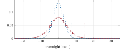
At ten to four a stock market maker is long a basket of forty names it never chose. Its clients sold into a falling afternoon, its quotes leaned against each position as the models of chapters 3 and 4 say they should, and still the book holds $1.6 million of stock, $830 000 of it in index-equivalent exposure. It can sell the stocks, sell the index future against them, or keep them overnight and start tomorrow long. In this chapter’s simulated market, selling the stocks costs $440; selling the future costs $83 and leaves an overnight standard deviation of $3 100; keeping the book leaves a one-in-a-hundred overnight loss of $14 800. During the day the same question arises every few seconds, and answering it at every move costs 14% of the spread the desk earns.

11.1 Choosing the hedge instrument

A market maker’s inventory is a by-product: it holds what clients sold to it. The inventory models of chapters 3 and 4 manage it through the quotes, which cost nothing but act slowly. A hedge acts at once but crosses a spread.

Definition 11.1 (Hedge instrument)

A hedge instrument is a security a market maker trades, not to earn a spread but to offset the risk of positions it acquired by making markets; it is chosen for the cost of trading it and for how much of the positions’ risk it removes.

The choice is between instruments that remove different parts of the risk at different prices. In a one-factor model, name $i$ has price $S_i$ , a beta $\beta_i$ to the market factor and an idiosyncratic daily volatility $\sigma_i$ ; the factor has daily volatility $\sigma_F$ and the index future tracks it.

Definition 11.2 (Delta-equivalent inventory)

The delta-equivalent inventory of a book is its exposure expressed in one reference instrument: each position’s value times its sensitivity to the reference, summed across instruments. Against an index, a book of stocks $q_i$ has

D=\sum_i q_i\,S_i\,\beta_i

dollars of index exposure; an ETF counts with its own beta, an option with its delta times its underlying’s beta.

The book’s daily variance is $D^2\sigma_F^2+\sum_i (q_iS_i\sigma_i)^2$ . Selling $D$ dollars of the future removes the first term at a cost $c_F|D|$ , with $c_F$ the future’s cost per dollar traded; trading every stock back to zero removes both at a cost $c_S\sum_i|q_iS_i|$ . With a charge $\lambda$ on each squared dollar of variance held for a horizon $h$ , the choice compares three numbers (Listing 11.1):

\lambda h\,\bigl(D^2\sigma_F^2+\textstyle\sum_i(q_iS_i\sigma_i)^2\bigr),\qquad c_F|D|+\lambda h\textstyle\sum_i(q_iS_i\sigma_i)^2,\qquad c_S\textstyle\sum_i|q_iS_i|.

The future wins when the book is concentrated in the factor and large, the stocks when the idiosyncratic risk is large or the horizon long, and doing nothing when the book is small. A future also brings risks the one-factor model omits: its basis to the cash index, the book’s betas estimated with error, and, for a book of stocks outside the index, a factor exposure the future does not match. Chapter 9 of One Quant Book 9 treats the estimated hedge ratio.

11.2 Partial hedging and hedge triggers

Hedging is rarely all or nothing. If the only cost is proportional, the one-period problem has a closed form.

Proposition 11.3 (The dead zone)

Selling $x$ dollars of the future against an exposure $D$ at cost $c_F|x|$ with a risk charge $\lambda\sigma_F^2(D-x)^2$ is optimal at

x^\ast=\operatorname{sign}(D)\,\max\Bigl(|D|-\frac{c_F}{2\lambda\sigma_F^2},\,0\Bigr):

the market maker hedges down to the edge of a dead zone of half-width $c_F/(2\lambda\sigma_F^2)$ and not inside it.

Proof. For $0<x<D$ the derivative of $c_Fx+\lambda\sigma_F^2(D-x)^2$ is $c_F-2\lambda\sigma_F^2(D-x)$ , zero at $D-x=c_F/(2\lambda\sigma_F^2)$ ; the objective is convex, and no hedge beyond $D$ or of the opposite sign helps. If $|D|$ is inside the half-width, the derivative at $x=0$ is already non-negative. ∎

Over a day, the exposure moves continuously as fills arrive, and the one-period answer becomes a band: do nothing while the unhedged exposure is inside $\pm b$ , trade back to the edge when it leaves. One Quant Book 4, chapter 10 derives the optimal band for an exposure that diffuses with volatility $\sigma_D$ , a running risk charge $\gamma X^2$ and a proportional cost $c$ : $b^\ast=\bigl(3c\sigma_D^2/(4\gamma)\bigr)^{1/3}$ . Here $\gamma=\lambda\sigma_F^2$ . The cube root makes the band robust: doubling the cost widens it by 26%.

A hedge trigger may also be an event rather than a level: a large fill, a fill from a client known to be informed, or a move in the market that makes the exposure’s risk jump. The discipline is the same: each hedge must be worth more in risk removed than it costs.

11.3 Inventory across correlated books

A firm that makes markets in the index’s stocks, its ETFs and its futures holds one factor exposure spread across books. Netting the delta-equivalent inventories before hedging is the cheapest hedge there is: a long in one book offsets a short in another, and the firm hedges only the sum. The desk that makes markets in ETFs (chapter 12) can often hedge with its own stock inventories; the options desk’s delta (chapter 19) adds to the same number.

Netting has two conditions. The books must be marked and summed in near real time, which is an engineering problem; and the residual risks that netting leaves (idiosyncratic, basis, time zone) must stay inside each book’s own limits.

The empirical record says inventory matters to prices and to liquidity. In twelve years of daily New York Stock Exchange specialist data from 1994 to 2005, Hendershott and Menkveld measured price pressures from intermediaries’ inventory of 49 basis points on average, with a half life of 0.92 days: 17 basis points and 0.54 days in the largest stocks, 118 basis points and 2.11 days in the smallest. Comerton-Forde, Hendershott, Jones, Moulton and Seasholes found in eleven years of the same specialists’ data that market-wide and firm-level spreads widen when specialists hold large positions or lose money, most strongly when inventories are big or results poor. And the high-frequency market maker Menkveld studied in 2013 earned a profit on the spread and lost on its positions: of € 1.55 a trade earned on the spread net of fees, € 0.68 went on positioning.

11.4 End of day and overnight

Definition 11.4 (End-of-day flattening)

End-of-day flattening is the reduction of a market maker’s positions towards zero before the close, through its quotes, through orders in the continuous market or in the closing auction, or by hedging what remains with an instrument that trades overnight.

The night changes the problem: the stocks cannot be traded until the open, the gap at the open is not a diffusion but a jump with fat tails, and the book has no spread income to set against it. Four ways to flatten, from cheapest to dearest:

Through the quotes. Skew harder in the last hour. In the tutorial, quotes skewed four times harder from 15:00 halve the gross book at the close, $1.32 million to $670 000, while the desk trades the same number of fills.
In the closing auction. No spread to cross, a single price; the risk is the auction’s own imbalance, and a large order moves the close (One Quant Book 1, chapter 13).
In the continuous market before the close: the half-spread plus impact.
Keep the stocks and sell the future overnight: the factor risk goes, the idiosyncratic gaps stay.

Hedging cost against intraday risk (the one-minute P&L’s standard deviation scaled to a day) for seven rules: no hedge, the future kept within half a contract of the book’s delta-equivalent inventory, the future outside no-trade bands of $100 000 to $1 million, and every name traded back to $20 000 in its own stock. Forty names, ten simulated days, spread income $46 800 a day. Data: hf_hedging.frontier. — **Figure 11.1.** Hedging cost against intraday risk (the one-minute P&L’s standard deviation scaled to a day) for seven rules: no hedge, the future kept within half a contract of the book’s delta-equivalent inventory, the future outside no-trade bands of $100 000 to $1 million, and every name traded back to $20 000 in its own stock. Forty names, ten simulated days, spread income $46 800 a day. Data: `hf_hedging.frontier`.

11.5 Tutorial: forty names, one factor, one future

Goal. Measure what each hedging rule costs and what risk it leaves on a simulated day of fills across forty names, then take the ten-to-four decision. End state: Figures 11.1 and 11.2 and the table of the ten-to-four decision.

The day. firm.mmhedge.FlowDay draws forty names (prices $20–150, betas 0.6–1.4, idiosyncratic volatility 1–2% a day, factor 1%), 0.05 fills a second per name of 100 shares at a half-spread of one cent, quotes skewed against inventory, and clients who sell after the factor falls (a tilt of 0.15 per standard deviation of the last minute’s move). The tilt makes the names’ inventories move together: the book’s delta-equivalent exposure has a daily volatility of $2.5 million. Simulating fills rather than forty full order books keeps the day at a fraction of a second; chapter 1’s harness is the tool when fills depend on the book.

The choice of instrument (Listing 11.1).

def choose(q, p, beta, sf, se, c_fut: float, c_stk: float, lam: float, horizon: float = 1.0) -> dict:
    """Hedge-instrument choice for a book held over `horizon` days: cost plus lam times the variance left.
    c_fut and c_stk are costs per dollar traded (half-spread plus fees)."""
    x = np.asarray(q) * np.asarray(p)
    d = delta_equivalent(q, p, beta)
    out = {"none": lam * horizon * book_var(q, p, beta, sf, se),
           "future": c_fut * abs(d) + lam * horizon * book_var(q, p, beta, sf, se, hedge=d),
           "stocks": c_stk * float(np.sum(np.abs(x)))}
    out["best"] = min(("none", "future", "stocks"), key=out.get)
    return out

Listing 11.1. Cost plus the charge on the variance left, for the three choices. code/firm/mmhedge/firm_mmhedge.py

The rules on the future: within half a contract ($50 000 notional), or a no-trade band.

def hedge_future(D, rule: str, band: float = 0.0, notional: float = 50000.0, c: float = 0.00005):
    """Future position (dollars, sold against a long exposure) along a path of delta-equivalent exposures D.
    'zero' keeps the unhedged exposure within half a contract; 'band' trades back to +-band when |D - H| > band.
    Returns (H path, cost in dollars, contracts traded)."""
    H = np.zeros(len(D))
    h, cost, traded = 0.0, 0.0, 0
    for t, d in enumerate(D):
        x = d - h
        if rule == "zero" and abs(x) > 0.5 * notional:
            k = int(round(x / notional))
        elif rule == "band" and abs(x) > band + 0.5 * notional:
            k = int(round((x - math.copysign(band, x)) / notional))
        else:
            k = 0
        if k:
            h += k * notional
            cost += c * abs(k) * notional
            traded += abs(k)
        H[t] = h
    return H, cost, traded

Listing 11.2. The future position along the day’s exposure, and what it cost. code/firm/mmhedge/firm_mmhedge.py

The frontier. Ten days, seven rules, future at half a basis point a dollar, stocks at 1.7 basis points (Figure 11.1).
Ten to four. Take the book at 15:50 of the first day and compare flattening in the last ten minutes (half-spread plus square-root impact), selling the future overnight (in and out: one basis point) and keeping it, with Student- $t$ gaps of four degrees of freedom (factor 0.6%, names 1%).

What to change next. Add a basis between the future and the factor; estimate the betas from a month of simulated returns instead of using the true ones; net a second book (an ETF) into $D$ .

The frontier (Figure 11.1): with no hedge, intraday risk is $8 540 a day. Keeping the future within half a contract halves it to $4 410 but trades 2 682 contracts and costs $6 700 a day, 14% of the spread income. A band of $250 000 leaves $4 760 of risk for $1 880. The stocks remove the idiosyncratic risk too ($2 525) for $12 760. With a charge of $\lambda=10^{-4}$ per squared dollar, the band of $250 000 scores best ($42 570 of spread income less costs and charge, against $39 640 unhedged and $38 260 for the future at every move), and the formula’s band is $284 000.

Overnight loss of the book held at 15:50 ($1.57 million gross, $834 000 delta-equivalent), kept as it is or with $834 000 of future sold, in bins of $1 000; Student-t gaps with four degrees of freedom, factor 0.6% and names 1% a night; 200 000 draws. Dotted lines: the 99% quantiles, $14 780 and $7 360. Data: hf_hedging.ten_to_four. — **Figure 11.2.** Overnight loss of the book held at 15:50 ($1.57 million gross, $834 000 delta-equivalent), kept as it is or with $834 000 of future sold, in bins of $1 000; Student- $t$ gaps with four degrees of freedom, factor 0.6% and names 1% a night; 200 000 draws. Dotted lines: the 99% quantiles, $14 780 and $7 360. Data: `hf_hedging.ten_to_four`.

at 15:50	cost	overnight s.d.	99% loss	99% expected shortfall
flatten in the last ten minutes	$438	0	0	0
sell the future overnight	$83	$3 086	$7 358	$8 813
keep	0	$5 879	$14 776	$19 795

With the same charge, the three choices score $438, $1 035 and $3 454: flattening wins, because the idiosyncratic gaps the future cannot remove are charged at a night’s variance with no spread to earn against them. Skewing the quotes from 15:00 would have halved the flattening bill ($163 against $381 on average over the ten days).

11.6 Build: the hedging module

Purpose. Express a market maker’s positions as one factor exposure, choose what to hedge with, and apply band, trigger and end-of-day rules.

Interface. delta_equivalent, book_var, choose(q, p, beta, sf, se, c_fut, c_stk, lam, horizon), partial_hedge, optimal_band (from firm.impulse), FlowDay(n, seed) with inventory(stock_band, c_stk, eod_from, eod_skew), hedge_future(D, rule, band, notional, c), day_pnl, overnight, flatten_cost.

Rules. Costs per dollar traded; the future trades in whole contracts; the band’s edge, not zero, is the target after a trigger; overnight gaps are fat-tailed.

Acceptance tests. code/firm/mmhedge/tests/: exposure and variance by hand and the choice in three constructed cases; the dead zone is the numerical argmin; the future rules keep the exposure within their bounds and the band trades a fifth as much; the tilt makes names co-move and the stock band caps every name; overnight standard deviation matches the formula; flattening cost by hand; the band matches the closed form; a harder skew from 15:00 halves the book at the close.

Stretch. Basis and beta estimation error; several books netted; a closing-auction flattening with imbalance risk.

Sources and further reading

T. Hendershott, A. J. Menkveld, Price pressures, Journal of Financial Economics 114(3), 2014, 405–423.
C. Comerton-Forde, T. Hendershott, C. M. Jones, P. C. Moulton, M. S. Seasholes, Time variation in liquidity: the role of market-maker inventories and revenues, Journal of Finance 65(1), 2010, 295–331.
A. J. Menkveld, High frequency trading and the new market makers, Journal of Financial Markets 16(4), 2013, 712–740.

11.7 Exercises

Exercise 11.1 ★

A book is long 1 000 shares of a $50 stock with beta 1.2 and short 500 shares of a $100 stock with beta 0.8. What is its delta-equivalent inventory, and how many $50 000 futures does the half-contract rule sell?

Solution

Solution of Exercise 11.1.

$D=1\,000\times50\times1.2-500\times100\times0.8=60\,000-40\,000=\$20\,000$ . It is less than half a contract ($25 000): no future is sold.

Exercise 11.2 ★

With $c_F=0.5$ basis point, $\lambda=10^{-4}$ and $\sigma_F=1\%$ , what is the dead zone’s half-width, and how much of an $833 747 exposure is hedged?

Solution

Solution of Exercise 11.2.

$c_F/(2\lambda\sigma_F^2)=0.00005/(2\times10^{-4}\times10^{-4})=\$2\,500$ ; the hedge is $833\,747-2\,500=\$831\,247$ .

Exercise 11.3 ★

What does it cost to sell $833 747 of future at 15:50 and buy it back at the open, at 0.5 basis point each way?

Solution

Solution of Exercise 11.3.

$2\times0.00005\times833\,747\approx\$83$ .

Exercise 11.4 ★★

The future removes the factor risk. Why does the hedged book still have an overnight standard deviation of $3 086?

Solution

Solution of Exercise 11.4.

The idiosyncratic gaps: each name moves by its own news overnight (1% here, fat-tailed), and $\sqrt{\sum_i(q_iS_i\sigma_i)^2}$ over forty positions of about $40 000 is about $3 000. Only trading the stocks removes it.

Exercise 11.5 ★★

Compute the optimal band at $\lambda=10^{-5}$ , $3\times10^{-5}$ and $10^{-4}$ with $\sigma_D=\$2.476$ million a day, and explain why the band narrows as risk aversion rises.

Solution

Solution of Exercise 11.5.

$b^\ast=\bigl(3c\sigma_D^2/(4\lambda\sigma_F^2)\bigr)^{1/3}$ : $613 000, $425 000 and $284 000. A higher charge on variance makes unhedged exposure dearer relative to the cost of trading, so the desk tolerates less of it before hedging; the cube root makes the band change slowly.

Exercise 11.6 ★★

Skewing the quotes harder from 15:00 halves the book at the close. Why is it nearly free, and when would it not be?

Solution

Solution of Exercise 11.6.

The desk still earns its half-spread on every fill; it only tilts which side trades, and clients on the favoured side cross a quote that is a little better for them. It is not free when the flow is one-sided (everyone sells at 15:30), when the skew moves the quote through the far touch and the desk pays the spread, or when the book is too large for the remaining hour’s flow.

Exercise 11.7 ★★★

Coding. Double the future’s cost (frontier(1e-4)). Which simulated band scores best, and what does the formula say?

Solution

Solution of Exercise 11.7.

With the future at one basis point a dollar the formula’s band is $358 000 at $\lambda=10^{-4}$ ; among the simulated bands, $500 000 scores best ($41 540, against $40 680 at $250 000 and $40 490 at $1 million), and hedging at every move falls to $31 560. The optimum moves out by about the cube root of two.

Exercise 11.8 ★★★

Find the flaw. “We sell a future every time the book’s beta moves by one contract. That minimises our risk, so it must be the right policy.”

Solution

Solution of Exercise 11.8.

Minimising risk is not the objective; risk has a price and so does hedging. The rule trades 2 682 contracts a day for $6 700, 14% of the spread income, and removes only slightly more risk than a $250 000 band that costs $1 880. It also leaves the idiosyncratic risk untouched.

11.8 Problem: Forty Names at Ten to Four

Problem 11.1

Weekend problem — forty names at ten to four

A stock market maker ends its day long a basket it did not choose and must decide how to hedge during the day and what to hold overnight.

Part I — The exposure.

Define a hedge instrument and the costs that choose it.
Define the delta-equivalent inventory of a book of stocks against an index.
Write the book’s daily variance in the one-factor model.
Why do clients who sell into a falling market make a market maker’s names co-move?

Part II — Rules.

State and prove the dead zone (Proposition 11.3).
Give the optimal band and its value at $\lambda=10^{-4}$ .
Name three risks of a future hedge that the one-factor model omits.
Why net across books before hedging, and on what conditions?

Part III — Measurements.

Give the cost and intraday risk of the four main rules.
Which rule scores best at $\lambda=10^{-4}$ , and how close is the formula?
What did the empirical studies find about inventory and prices, and inventory and spreads?
What did Menkveld’s market maker earn on the spread and lose on positions?

Part IV — The verdict.

State the named result: the cost and residual risk of the three choices at 15:50, and the overnight loss distribution of keeping the book.
Which choice wins with the same charge, and why?
Define end-of-day flattening and list its four routes.
What does skewing from 15:00 change in the flattening bill?
When would keeping the book overnight be right?
How does the answer change if the betas are estimated with error?
What would an options book add to the delta-equivalent inventory?
In one sentence: when is a hedge worth it?

Solution

Solution of Problem 11.1.

See Definition 11.1: the cost of trading it and the share of the risk it removes.
See Definition 11.2: $D=\sum_iq_iS_i\beta_i$ .
$D^2\sigma_F^2+\sum_i(q_iS_i\sigma_i)^2$ .
After a fall, fills in every name tend to make the desk long at once: the inventories share the factor’s sign.
See Proposition 11.3 and its proof.
$b^\ast=\bigl(3c\sigma_D^2/(4\lambda\sigma_F^2)\bigr)^{1/3}$ , $284 000.
Basis between the future and the index, betas estimated with error, and stocks outside the index.
Offsetting positions cancel before anyone pays a spread; the books must be summed in near real time and each residual must stay within its own limits.
None: $0 and $8 540 a day; future at every move: $6 700 and $4 410; band $250 000: $1 880 and $4 760; stocks: $12 760 and $2 525.
The $250 000 band ($42 570); the formula gives $284 000, between the two best simulated bands.
Price pressures of 49 basis points with a half life of 0.92 days on average (Hendershott and Menkveld); spreads wider when specialists hold large positions or lose money (Comerton-Forde and co-authors).
€ 1.55 a trade on the spread net of fees; € 0.68 lost on positions.
Flatten: $438 and no risk; future overnight: $83, standard deviation $3 086, 99% loss $7 358, expected shortfall $8 813; keep: 99% loss $14 776, expected shortfall $19 795, standard deviation $5 879.
Flattening ($438 against $1 035 and $3 454): the idiosyncratic risk left by the future costs more in a night than the flattening does.
See Definition 11.4: through the quotes, the closing auction, the continuous market, the future overnight.
It halves the book at the close and the bill, from $381 to $163 on average.
When the book is small relative to the cost of flattening, when tomorrow’s flow is expected to unwind it, or when the positions are a hedge of something else the firm holds.
The future hedge leaves a factor residual proportional to the beta errors; the choice tilts towards stocks or towards a smaller hedge.
Each option’s delta times its underlying’s beta and price; gamma makes the number move with the market.
When the risk it removes is worth more, at the firm’s price of risk, than the spread and fees it pays.

11.9 Interview questions

Interview question 11.1 ★ trader

You are long $5 million of bank stocks at 15:55. What are your options, and which do you take?

Solution

Solution of Interview question 11.1.

Sell in the closing auction, sell the stocks now, sell a bank ETF or the index future against them, or keep. The sector ETF removes more of the sector risk than the index future; the closing auction avoids the spread but is a single price that a large order moves. The answer depends on the size relative to the names’ closing volume and on the desk’s limits.

What the interviewer is looking for: routes, costs, residual risk, size.

Interview question 11.2 ★★ researcher

How would you estimate the betas used to hedge a book of forty names with the index future, and how would you test the hedge?

Solution

Solution of Interview question 11.2.

Regress each name’s returns on the future’s over a window long enough to be stable and short enough to be current (with care for asynchronous closes); test by the variance of the hedged book out of sample, compared with the unhedged.

What the interviewer is looking for: estimation and an out-of-sample test.

Interview question 11.3 ★★ researcher

Why does a proportional cost produce a no-trade band, and a fixed cost a jump back to zero?

Solution

Solution of Interview question 11.3.

With a proportional cost, a small trade costs little, so the desk trades just enough to stay inside the band; with a fixed cost, each trade costs the same whatever its size, so when the desk trades it goes all the way to the best position.

What the interviewer is looking for: marginal versus fixed cost.

Interview question 11.4 ★★ risk

Three desks each report a small index exposure within limits. What could go wrong at the firm level?

Solution

Solution of Interview question 11.4.

The three exposures may have the same sign and add up to a firm-wide exposure beyond any limit; or they may offset each other, and each desk hedges anyway, paying for three hedges of nothing. The firm needs the sum in real time.

What the interviewer is looking for: aggregation across desks.

Interview question 11.5 ★★ developer

Design the service that computes the firm’s delta-equivalent inventory in real time across stocks, ETFs, futures and options.

Solution

Solution of Interview question 11.5.

Positions from every book’s fills (drop copies), a shared table of betas and deltas updated on a timer, prices from the fair-value service, a sum updated per fill; publish to the hedger and risk; reconcile against the end-of-day positions.

What the interviewer is looking for: event-driven aggregation with reference data.

Interview question 11.6 ★★★ researcher

Derive the half-width of the dead zone and explain how it changes with the horizon of the hedge.

Solution

Solution of Interview question 11.6.

Minimise $c|x|+\lambda h\sigma_F^2(D-x)^2$ : the half-width is $c/(2\lambda h\sigma_F^2)$ , shrinking as the horizon $h$ grows, since the variance avoided grows with the time the exposure is held while the cost of the trade does not.

What the interviewer is looking for: the first-order condition and the horizon.

Terms defined in this chapter

See all 2333 terms in the glossary