Market Making and High-Frequency Trading · Market making

4Extensions of the Inventory Framework

The exact solution of chapter 3 tells a market maker holding four units to offer them below the mid. Real market makers stop buying instead: they bound the inventory. They also hold several correlated books at once, they know something about where the price is going, and they know that the next trade is more likely to come from someone who knows more than they do. Each of these enters the same linear system. In this chapter’s simulations, quoting two assets whose prices are correlated 0.8 as one book instead of two carries 21% less inventory risk for the same expected profit; a market maker who knows the drift holds the position the formula targets; and one whose fills are followed by an adverse move does best by widening each quote by half that move, not by all of it.

4.1 Inventory bounds and the asymptotic solution

Definition 4.1 (Inventory bound)

An inventory bound $\bar q$ is a hard limit on the market maker’s position: at $q=\bar q$ it does not bid, at $q=-\bar q$ it does not offer, so that $|q_t|\le\bar q$ at all times.

The bound is part of the state space of Proposition 3.6 of chapter 3, which is why that solution was exact on a finite grid. Its first use is practical: whatever the model says, the position cannot run away. Its second is analytical: on a finite grid the long-horizon behaviour of the solution is an eigenvector problem.

Proposition 4.2 (The stationary quotes)

As $T-t\to\infty$ , the depths of chapter 3’s running-penalty model converge to time-independent depths given by the same formulas with $h=\tfrac1k\ln v$ , where $v$ is the eigenvector of the largest eigenvalue of $M$ .

Proof. $M$ is symmetric with positive off-diagonal entries next to the diagonal, so its largest eigenvalue $\mu_1$ is simple and its eigenvector $v$ can be taken positive (Perron–Frobenius). Then $\omega(t)=e^{M(T-t)}z=\sum_ie^{\mu_i(T-t)}(v_i^\top z)v_i$ is dominated by the first term as $T-t\to\infty$ , since $v^\top z>0$ . The depths depend on $\omega$ only through ratios across $q$ , so the factor $e^{\mu_1(T-t)}(v^\top z)$ drops out. ∎

In the chapter 3 parameters ( $A=140$ , $k=1.5$ , $\phi=0.5$ ) a horizon of one unit of time is already long: the depths at its start agree with the stationary ones to eight decimals. Guéant, Lehalle and Fernandez-Tapia solved the exponential-utility version the same way and approximated the eigenvector in closed form. The same approximation for the running penalty gives a formula simple enough to put in a pricing function.

Proposition 4.3 (Closed-form stationary quotes)

If the eigenvector is approximately Gaussian, $v_q\propto e^{-\beta q^2/2}$ with $\beta$ small, then $\beta^2=\phi ke/A$ and, with $c=\beta/k=\sqrt{\phi e/(Ak)}$ ,

\delta^b(q)\simeq\frac1k+\frac{2q+1}{2}\,c,\qquad \delta^a(q)\simeq\frac1k-\frac{2q-1}{2}\,c .

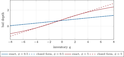
Proof. The eigenvalue equation is $Ae^{-1}(v_{q-1}+v_{q+1})-\phi kq^2v_q=\mu_1v_q$ . With the Gaussian ansatz, $v_{q\pm1}/v_q=e^{-\beta(\pm2q+1)/2}$ , whose sum is $2e^{-\beta/2}\cosh(\beta q)\simeq2-\beta+\beta^2q^2$ to second order. Matching the terms in $q^2$ gives $Ae^{-1}\beta^2=\phi k$ . Then $h(q)-h(q\pm1)=\tfrac1k\ln(v_q/v_{q\pm1})=\tfrac{\beta}{2k}(\pm2q+1)$ . ∎

Each unit of inventory shifts both quotes by $c$ , and the spread stays $2/k+c$ . For $\gamma\to0$ with $\phi=\tfrac12\gamma\sigma^2$ , the Guéant–Lehalle–Fernandez-Tapia formula reduces to this one. The approximation needs $\beta$ small, that is a penalty small against the fill rate:

bid depth, $\phi=0.5$	$q=0$	$q=1$	$q=2$	$q=3$	worst gap, $\|q\|\le10$
exact, stationary	0.708	0.790	0.872	0.953
closed form	0.707	0.787	0.868	0.948	0.034
worst gap for $\phi=5$ / $\phi=50$					0.70 / 5.0

Figure 4.1 shows the failure at $\phi=5$ : the exact depths curve at large inventories, where the eigenvector is far from Gaussian; the straight line does not.

Stationary bid depth against inventory: exact (eigenvector) and closed form, for two running penalties (A=140, k=1.5, inventory within ±20). Data: firm.multimm. — **Figure 4.1.** Stationary bid depth against inventory: exact (eigenvector) and closed form, for two running penalties ( $A=140$ , $k=1.5$ , inventory within $\pm20$ ). Data: `firm.multimm`.

4.2 Many assets and correlated inventory

Definition 4.4 (Multi-asset market making)

Multi-asset market making quotes several instruments from one inventory vector $q\in\mathbb Z^d$ and one risk charge on the whole book, $\phi\,q^\top\Sigma q$ per unit of time, with $\Sigma$ the covariance of the instruments’ price changes, so that each quote depends on the inventory of every instrument.

Proposition 4.5 (Exact multi-asset quotes)

If the instruments share $A$ and $k$ , the substitution $h=\tfrac1k\ln\omega$ turns the problem on the grid $\{-\bar q,\dots,\bar q\}^d$ into the linear system $\partial_t\omega+M\omega=0$ , with $M_{q,q}=-\phi k\,q^\top\Sigma q$ and $Ae^{-1}$ between neighbouring inventories $q\pm e_i$ ; the depths of instrument $i$ are $\delta^{b,a}_i(q)=\tfrac1k+h(q)-h(q\pm e_i)$ , and Proposition 4.2 holds on the grid.

Proof. As in chapter 3, instrument by instrument: each side’s supremum contributes

\tfrac1k\,Ae^{-1}\,e^{k(h(q\pm e_i)-h(q))},

which is linear in $\omega$ after the substitution because every instrument has the same $k$ . ∎

The shared $k$ is the price of exactness; with different $k_i$ the system is no longer linear and the multi-asset literature (Guéant 2017) turns to quadratic approximations of the value function. The grid has $(2\bar q+1)^d$ points, 289 for two instruments with $\bar q=8$ : fine for a pair, not for a hundred names.

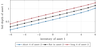
Correlation creates a cross-skew. Under the joint policy (Figure 4.2), a market maker short four units of the second instrument bids for the first at 0.572 from the mid when flat in it, against 0.700 when flat in both: a long position in the first hedges the short in the second. Asset by asset, the bid would be 0.700 whatever the other position.

The joint policy’s bid depth for asset 1 against its own inventory, for three inventories of asset 2 (two assets with price correlation 0.8, penalty =0.1 on q q, A=140, k=1.5, =2). Data: hf_extensions.cross_skew. — **Figure 4.2.** The joint policy’s bid depth for asset 1 against its own inventory, for three inventories of asset 2 (two assets with price correlation 0.8, penalty $\phi=0.1$ on $q^\top\Sigma q$ , $A=140$ , $k=1.5$ , $\sigma=2$ ). 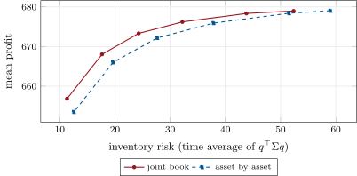Data: `hf_extensions.cross_skew`.

The cross-skew pays. On 1 000 simulated paths of five units of time, with the two mids correlated 0.8, the joint policy and the asset-by-asset policy (the same penalty applied to each asset’s own variance) earn almost the same, but the joint book carries less inventory risk, measured as the time average of $q^\top\Sigma q$ (Figure 4.3). At the joint policy’s mean profit for $\phi=0.1$ , 673.3, the asset-by-asset frontier carries 30.8 units of inventory risk and the joint policy 24.3: 21% less. Across the six penalties the reduction runs from 10% to 22%.

Mean profit against inventory risk for two assets correlated 0.8, quoted as one book or asset by asset, for penalties from 0.01 (right) to 0.5 (left); 1 000 common paths of five units of time. Data: hf_extensions.frontier2. — **Figure 4.3.** Mean profit against inventory risk for two assets correlated 0.8, quoted as one book or asset by asset, for penalties $\phi$ from 0.01 (right) to 0.5 (left); 1 000 common paths of five units of time. Data: `hf_extensions.frontier2`.

4.3 Signals and drift inside the control problem

Definition 4.6 (Drift-adjusted quoting)

Drift-adjusted quoting solves the market maker’s control problem with the forecast drift $\mu$ of the mid inside it, so that the forecast shifts the quotes through the value of holding inventory rather than being added to them as a separate skew.

With $dS_t=\mu\,dt+\sigma\,dW_t$ , holding $q$ earns $\mu q$ per unit of time, and the running reward is $\mu q-\phi q^2=-\phi(q-q_0)^2+\text{const}$ with $q_0=\mu/(2\phi)$ .

Proposition 4.7 (A drift sets a target position)

With a constant drift $\mu$ , the diagonal of $M$ becomes $k(\mu q-\phi q^2)$ , and in the closed form of Proposition 4.3 the market maker quotes as if its inventory were $q-q_0$ : it targets the position $q_0=\mu/(2\phi)$ .

Proof. The running reward enters $M$ ’s diagonal multiplied by $k$ , as $-\phi q^2$ did. Completing the square, the eigenvalue equation of Proposition 4.3 holds with $q$ replaced by $q-q_0$ up to a constant absorbed in $\mu_1$ . ∎

Guéant, Lehalle and Fernandez-Tapia’s formula with a drift has the same shape, a shift of the inventory by $\mu/(\gamma\sigma^2)$ , which is $q_0$ for $\phi=\tfrac12\gamma\sigma^2$ . Cartea and Wang put a stochastic alpha signal inside the problem in the same spirit. In the simulation with $\mu=2$ , $\phi=0.5$ (so $q_0=2$ ), the drift-adjusted market maker holds 1.97 units on average and earns 355.6, against 335.7 for the market maker that ignores the drift and stays flat: 5.9% more, for a standard deviation of 18.0 instead of 15.8. The forecast is worth money only through the position it makes the market maker hold; chapter 7 builds such forecasts at the horizon of seconds.

4.4 Adverse selection inside the model

Adverse selection enters the model in two ways, and they call for different widenings.

Proposition 4.8 (Widen by the cost, or by half the move)

(i) If each fill costs an expected $\varepsilon$ (the fill price is on average $\varepsilon$ worse than the mid), the off-diagonal of $M$ becomes $Ae^{-1-k\varepsilon}$ and both optimal depths increase by $\varepsilon$ at every inventory. (ii) If instead the mid moves permanently by $\xi$ against the market maker after each of its fills, the optimal depths are those of (i) with $\varepsilon=\xi/2$ .

Proof. (i) Each supremum becomes $\sup_\delta Ae^{-k\delta}(\delta-\varepsilon+\Delta h)$ : the optimum is $1/k+\varepsilon-\Delta h$ and its value carries a factor $e^{-k\varepsilon}$ . (ii) After a bid fill the whole position $q+1$ is revalued by $-\xi$ , after an ask fill $q-1$ by $+\xi$ : the brackets are $\delta-\xi(q+1)+h(q+1)-h(q)$ and $\delta+\xi(q-1)+h(q-1)-h(q)$ . With $h(q)=\tilde h(q)+\tfrac12\xi q^2$ both become $\delta-\tfrac12\xi+\Delta\tilde h$ , the problem (i) for $\tilde h$ with $\varepsilon=\xi/2$ , and the depths expressed through $\tilde h$ are those of (i). ∎

Half, because the move that hurts the unit just traded also revalues the rest of the position, and on average the position the fill leaves is on the right side of the move as often as on the wrong one. The simulation of (ii) with $\xi=0.3$ , $\phi=0.5$ agrees, provided the time step is fine enough:

widening of each depth	none	$\xi/2=0.15$	$\xi=0.3$
mean profit	262.7	267.2	258.9
profit less the penalty	253.1	258.6	251.2
fills	498	396	315
profit less the penalty, time step four times coarser	270.8	270.2	259.3

With the coarse step (0.005, when a flat quote has about a 24% chance of a fill per step), the unadjusted policy looked marginally best; divided by four, the step reproduces the proposition. The rule of One Quant Book 7 applies: a simulation that a named result leans on is rerun with a quarter of the time step.

4.5 Tutorial: one linear system, four extensions

Goal. Compute stationary, closed-form, multi-asset, drift-adjusted and adverse-selection-adjusted quotes from one construction, and test each in simulation. End state: the three tables and three figures of the chapter.

Stationary and closed form. The Perron eigenvector of $M$ gives the long-horizon depths; the Gaussian approximation gives the formula (Listing 4.1).

def stationary(A: float, k: float, phi: float, qmax: int, mu: float = 0.0, eps: float = 0.0):
    """Long-horizon depths: omega(t) tends to the eigenvector of the largest eigenvalue of M (symmetric), so the depths
    stop depending on time."""
    M, qs = _tridiag(A, k, phi, qmax, mu, eps)
    w, V = np.linalg.eigh(M)
    v = np.abs(V[:, -1])
    h = np.log(np.maximum(v / v.max(), 1e-300)) / k
    bid = np.full(len(qs), np.nan)
    ask = np.full(len(qs), np.nan)
    ask[1:] = 1.0 / k + eps + h[1:] - h[:-1]
    bid[:-1] = 1.0 / k + eps + h[:-1] - h[1:]
    return bid, ask


def asymptotic(A: float, k: float, phi: float, q, mu: float = 0.0, eps: float = 0.0):
    """Closed form of the stationary depths from a Gaussian eigenvector exp(-beta (q - q0)^2 / 2),
    beta^2 = phi k e / A."""
    q = np.asarray(q, float)
    c = math.sqrt(phi * math.e / (A * k))
    q0 = mu / (2.0 * phi) if phi > 0 else 0.0
    return 1.0 / k + eps + (2 * (q - q0) + 1) / 2 * c, 1.0 / k + eps - (2 * (q - q0) - 1) / 2 * c

Listing 4.1. Stationary depths from the eigenvector, and their closed form. code/firm/multimm/firm_multimm.py

Two assets. The same construction on the grid of inventory pairs (Listing 4.2); simulate_multi draws correlated mids.

    def __init__(self, A: float, k: float, phi: float, cov, qmax: int):
        cov = np.asarray(cov, float)
        d = cov.shape[0]
        side = 2 * qmax + 1
        grid = np.array(np.meshgrid(*[np.arange(-qmax, qmax + 1)] * d, indexing="ij")).reshape(d, -1).T
        n = len(grid)
        M = np.zeros((n, n))
        M[np.arange(n), np.arange(n)] = -phi * k * np.einsum("ni,ij,nj->n", grid, cov, grid)
        off = A * math.exp(-1.0)
        strides = [side ** (d - 1 - i) for i in range(d)]
        for i in range(d):
            ok = grid[:, i] < qmax
            src = np.flatnonzero(ok)
            M[src, src + strides[i]] = off
            M[src + strides[i], src] = off
        w, V = np.linalg.eigh(M)
        v = np.abs(V[:, -1])
        self.h = (np.log(np.maximum(v / v.max(), 1e-300)) / k).reshape([side] * d)
        self.k, self.qmax, self.d = k, qmax, d

Listing 4.2. The multi-asset linear system and its eigenvector. code/firm/multimm/firm_multimm.py

Frontiers. hf_extensions.frontier2() runs both policies for six penalties on 1 000 common paths; equal_capture() interpolates the asset-by-asset frontier at each joint mean.
Drift and adverse selection. drift_case(adjust) and adverse_case(adjust, dt).

What to change next. Give the two assets different fill rates and compare the grid solution with a quadratic approximation; make the drift switch sign at random (a Markov signal) and add it to the state.

4.6 Build: the multi-asset and signal extensions

Purpose. Long-horizon quotes that a production quoter can evaluate in microseconds (a table or a formula), for one or several instruments, with a drift and adverse selection inside the problem.

Interface. firm.multimm: stationary(A, k, phi, qmax, mu, eps), asymptotic(A, k, phi, q, mu, eps), MultiStationary(A, k, phi, cov, qmax).depths(q), simulate_multi(policy, T, dt, cov, A, k, paths, seed, qmax), table_policy; firm.invmm.CJSolution(…, mu, eps) for finite horizons.

Rules. The inventory bound is never breached. A permanent post-fill move $\xi$ is passed as $\varepsilon=\xi/2$ . Simulations that support a printed result are repeated with a quarter of the time step.

Acceptance tests. code/firm/multimm/tests/: the stationary depths equal the finite-horizon ones at the start of a long horizon; the closed form within 0.05 of the exact depths for a small penalty and its per-unit skew equal to $c$ ; a drift shifts the quotes by $q_0$ ; $\varepsilon$ shifts both closed-form depths by $\varepsilon$ ; two uncorrelated assets quote like two single assets; with correlation, a short position in one asset lowers the bid depth of the other; the simulator is deterministic and bounded.

Stretch. Different $k_i$ with a quadratic approximation of $h$ ; a Markov-modulated drift in the state.

Sources and further reading

O. Guéant, C.-A. Lehalle and J. Fernandez-Tapia, “Dealing with the inventory risk: a solution to the market making problem”, Mathematics and Financial Economics 7(4), 2013.
O. Guéant, “Optimal market making”, Applied Mathematical Finance 24(2), 2017.
Á. Cartea and Y. Wang, “Market making with alpha signals”, International Journal of Theoretical and Applied Finance 23(3), 2020.

4.7 Exercises

Exercise 4.1 ★

Compute $c=\sqrt{\phi e/(Ak)}$ for $A=140$ , $k=1.5$ , $\phi=0.5$ , and the closed-form bid and ask depths at $q=2$ .

Solution

Solution of Exercise 4.1.

$c=\sqrt{0.5e/210}=0.0804$ ; $\delta^b(2)=0.667+2.5c=0.868$ , $\delta^a(2)=0.667-1.5c=0.546$ .

Exercise 4.2 ★

A market maker with $\phi=0.5$ forecasts a drift of $\mu=1$ . What position does it target?

Solution

Solution of Exercise 4.2.

$q_0=\mu/(2\phi)=1$ unit.

Exercise 4.3 ★

How many grid points does the exact multi-asset solution need for three instruments with $\bar q=8$ , and for ten?

Solution

Solution of Exercise 4.3.

$17^3=4\,913$ points for three instruments; $17^{10}\approx2.0\times10^{12}$ for ten: the grid is out of reach, hence quadratic approximations.

Exercise 4.4 ★★

Show that the closed-form spread $\delta^a+\delta^b$ does not depend on inventory, and give it for the parameters of exercise 1.

Solution

Solution of Exercise 4.4.

$\delta^a+\delta^b=2/k+c\bigl((2q+1)-(2q-1)\bigr)/2=2/k+c$ , free of $q$ : $1.333+0.080=1.414$ .

Exercise 4.5 ★★

Why does the joint policy bid more aggressively for asset 1 when short asset 2, and would it do so if the correlation were negative?

Solution

Solution of Exercise 4.5.

With positive correlation, a long position in asset 1 offsets part of the variance of the short in asset 2, so buying asset 1 lowers the penalty $\phi q^\top\Sigma q$ . With negative correlation the offsetting position is a short in asset 1: the market maker would bid less and offer more aggressively.

Exercise 4.6 ★★

Explain in words why a permanent post-fill move $\xi$ calls for widening by $\xi/2$ rather than $\xi$ .

Solution

Solution of Exercise 4.6.

The move revalues the whole remaining position, not only the unit traded. After a bid fill the position is $q+1$ , after an ask fill $q-1$ ; averaged over the positions the market maker holds, the loss per fill beyond the unit itself cancels to a quadratic term in $q$ that the value function absorbs, and what remains is half the move per fill.

Exercise 4.7 ★★★

Coding. With stationary(140, 1.5, 0.5, 20, mu=2.0), give the bid and ask depths at $q=0$ and at $q=2$ , and compare them with the depths at $q=0$ without a drift.

Solution

Solution of Exercise 4.7.

At $q=0$ : bid 0.543, ask 0.872 (keen to buy); at $q=2$ : 0.708 on both sides, exactly the no-drift depths at $q=0$ . The drift moves the whole schedule by $q_0=2$ .

Exercise 4.8 ★★★

Find the flaw. “Our simulation shows that widening for adverse selection loses money, so we quote at the monopoly depth and ignore it.”

Solution

Solution of Exercise 4.8.

Three possible errors. Widening by the whole move instead of half of it (a permanent move revalues the position too); a time step coarse enough to change the answer (the chapter’s coarse step favoured no widening, the fine one half the move); and scoring on mean P&L while the policy maximises P&L less the penalty. Widen by half the permanent move, check with a quarter of the time step, and score the objective.

4.8 Problem: Two Books, One Risk

Problem 4.1

Weekend problem — two books, one risk

A desk makes markets in two instruments that move together and has a signal for one of them.

Part I — Bounds and the long horizon.

Define an inventory bound and say why it makes the long-horizon quotes an eigenvector problem.
Prove Proposition 4.2.
Derive the closed form of Proposition 4.3.
When is the closed form accurate? Give the worst gaps for $\phi=0.5$ , 5 and 50.

Part II — Two assets.

Define multi-asset market making and write the risk charge.
Why must the instruments share $k$ for the exact solution?
Give the cross-skew: asset 1’s bid depth at $q_1=0$ when short four, flat and long four of asset 2.
Describe the simulation and its measure of inventory risk.
State the named result: the reduction in inventory risk from quoting the two assets as one book, at equal mean profit, for $\phi=0.1$ , and its range across penalties.
Why is the reduction in P&L standard deviation much smaller than in inventory risk?

Part III — The signal.

Define drift-adjusted quoting.
Prove Proposition 4.7.
Give the simulated gain and average position with $\mu=2$ , $\phi=0.5$ .
What is the drift worth if the market maker’s bound is below $q_0$ ?

Part IV — Adverse selection.

Prove both parts of Proposition 4.8.
Give the simulated profit and penalised objective for no widening, $\xi/2$ and $\xi$ .
Why did the coarse time step point to no widening?
Which of the chapter’s four extensions would you implement first in a production quoter, and why?
How would you estimate $\xi$ from your own fills?
In one sentence: what do bounds, correlation, signals and adverse selection have in common in this framework?

Solution

Solution of Problem 4.1.

A hard limit $|q|\le\bar q$ ; it makes the state space finite, so the linear system has a largest eigenvalue that dominates as the horizon grows.
See Proposition 4.2 (Perron–Frobenius and the spectral decomposition of $e^{M(T-t)}$ ).
See Proposition 4.3.
When $\beta=\sqrt{\phi ke/A}$ is small; worst gaps for $|q|\le10$ : 0.034, 0.70 and 5.0.
One inventory vector and the charge $\phi q^\top\Sigma q$ on the whole book.
The substitution $h=\tfrac1k\ln\omega$ linearises every instrument’s term only if all share the same $k$ .
0.572, 0.700 and 0.828.
1 000 common paths of five units of time, mids correlated 0.8, six penalties; inventory risk is the time average of $q^\top\Sigma q$ .
21% less (24.3 against 30.8 at a mean profit of 673.3); 10% to 22% across penalties.
P&L variance also comes from the randomness of fills and spread capture, which quoting jointly does not change.
The drift inside the control problem, acting through the value of holding inventory.
See Proposition 4.7.
355.6 against 335.7 (5.9% more), holding 1.97 units on average against a target of 2.
Less: the market maker can only hold up to its bound, and the reward $-\phi(q-q_0)^2$ is then maximised at the bound.
See Proposition 4.8.
Profit 262.7, 267.2, 258.9; objective 253.1, 258.6, 251.2 for none, 0.15 and 0.3.
With a flat quote filled with probability about 0.24 per step, the discrete simulation departs from the continuous-time model the proposition solves; with a quarter of the step it agrees.
Adverse selection: it is present in every real market (chapter 1’s quoter lost its spread to it), and the adjustment is a constant per side.
Mark out one’s own fills at the horizon where the curve settles (One Quant Book 7, chapter 23): the settled mark-out is $\xi$ .
Each is a change to one matrix: its size (bounds, assets), its diagonal (penalties, drift) or its off-diagonal (adverse selection).

4.9 Interview questions

Interview question 4.1 ★ trader

You make markets in an index future and its exchange-traded fund. You are long the fund. How should that change your quotes in the future?

Solution

Solution of Interview question 4.1.

Being long the fund is being long the index: skew the future’s quotes as if you were already long it, keener to sell and less keen to buy, by the hedge ratio times your fund inventory.

What the interviewer is looking for: thinking in one book, with a hedge ratio.

Interview question 4.2 ★★ researcher

Why do the finite-horizon quotes stop depending on time far from the horizon?

Solution

Solution of Interview question 4.2.

The solution is $e^{M(T-t)}z$ ; far from the horizon the largest eigenvalue dominates, and the depths depend only on ratios of the dominant eigenvector.

What the interviewer is looking for: the spectral argument, or an ergodic-control intuition.

Interview question 4.3 ★★ researcher

Your fills are followed by a 0.3-tick adverse move on average. By how much do you widen, and what do you need to know first?

Solution

Solution of Interview question 4.3.

Whether the move is a cost on the unit (widen by 0.3) or a permanent move of the mid (widen by 0.15); measure the mark-out curve and where it settles, and check how much of the move reverts.

What the interviewer is looking for: the distinction and a measurement plan.

Interview question 4.4 ★★ developer

A quoter must evaluate its depths in under a microsecond. How do you deliver a model whose exact solution is an eigenvector problem?

Solution

Solution of Interview question 4.4.

Precompute: solve offline, store the depths in a table indexed by inventory (and a few signal buckets), or use the closed form; refresh the table when parameters change, off the hot path.

What the interviewer is looking for: precomputation and a lookup on the hot path.

Interview question 4.5 ★★ risk

A desk measures inventory risk instrument by instrument. What does it miss, and how would you measure it instead?

Solution

Solution of Interview question 4.5.

The correlation between positions: offsetting positions look risky and concentrated ones look diversified. Measure $q^\top\Sigma q$ (or a factor-model version) on the whole book.

What the interviewer is looking for: portfolio variance, not a sum of variances.

Interview question 4.6 ★★★ researcher

In a running-penalty market-making model, show that a constant drift $\mu$ makes the market maker target the position $\mu/(2\phi)$ .

Solution

Solution of Interview question 4.6.

The running reward $\mu q-\phi q^2=-\phi(q-\mu/(2\phi))^2+\mu^2/(4\phi)$ : the problem is the zero-drift one in the shifted variable $q-q_0$ , whose optimum centres the inventory at zero.

What the interviewer is looking for: completing the square.

Terms defined in this chapter

See all 2333 terms in the glossary