Market Making and High-Frequency Trading · Market making
21FX Market Making
A non-bank liquidity provider streams euro-dollar prices to a hundred banks, brokers and platforms at once, each with its own price; a trade on one of them is hedged, or not, within microseconds on another. In this chapter’s model, the stream’s last look lifts the capture on the most toxic tier from 0.13 to 0.20 basis point a request and lowers it on the others, for a third of all requests rejected; and internalising the flow instead of hedging it doubles the day’s result, but only if the stream’s skew brings offsetting trades back within a few hundred trades.
21.1 Principal electronic liquidity provision
Foreign exchange (One Quant Book 2, chapters 14 and 15) trades over the counter, in a web of venues: primary interdealer venues, electronic communication networks, single-dealer and multi-dealer platforms, and the liquidity aggregators of One Quant Book 10, chapter 21. Electronic market makers, banks and non-banks, quote as principals: they stream prices, take the other side of every trade they accept, and manage the inventory that results.
As of September 2026 — The size of the market
The BIS Triennial Central Bank Survey’s preliminary results, published on 30 September 2025, put FX trading at $9.6 trillion a day in April 2025. FX swaps remained the most traded instrument at $4 trillion a day; turnover in spot rose 42% and in outright forwards 60% since April 2022, to 31% and 19% of the total. The US dollar was on one side of 89% of all trades; sales desks in the United Kingdom, the United States, Singapore and Hong Kong accounted for 75%.
Chaboud, Chiquoine, Hjalmarsson and Vega studied the rise of algorithmic trading in the interdealer FX market with data that identified computer-generated activity. Algorithmic trading improved two measures of price efficiency, the frequency of triangular arbitrage opportunities and the autocorrelation of high-frequency returns; fewer arbitrage opportunities came mainly from computers taking liquidity, which may impose higher adverse selection costs on slower traders, and less autocorrelation from computers providing it.
21.2 Pricing from many venues
The provider’s fair price (chapter 2) combines the venues it sees, each with its own noise and its own delay. Weighting each venue’s mid by the inverse of its variance, the noise plus the variance the rate has accumulated since that venue last updated (Listing 21.1), beats the primary venue alone: in the chapter’s model of three venues (noise of 0.3, 0.6 and 0.8 basis point, updating every 1, 3 and 5 milliseconds on average), the consolidated price is 0.26 basis point from the true rate, the primary 0.30.
Definition 21.1 (Synthetic cross)
A synthetic cross is a price for a currency pair built from two pairs that share a currency, such as euro-yen from euro-dollar and dollar-yen, with its bid from the legs’ prices that the provider can hit and its offer from those it can lift.
With euro-dollar at 1.0850/1.0851 and dollar-yen at 150.20/150.21, the synthetic euro-yen is 162.967/162.993: 2.6 pips wide, the two legs’ spreads compounded. A provider that quotes the cross tighter than its synthetic must expect to internalise part of the flow, or hedge at the direct cross’s own market when that is cheaper.
21.3 Streams, tiers and last look
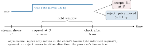
The provider streams a price to each client or platform, wider for tiers whose flow is more informed (One Quant Book 9, chapter 24 on client tiering). Last look (One Quant Book 2, chapter 15, where the FX Global Code’s principles for it are given) lets it hold a request for a few milliseconds and reject it if the price has moved. The chapter’s streams: tier 1 (banks and platforms, with fast arbitrage clients) at 0.3 basis point, 30% of its requests informed; tier 2 (brokers) at 0.5, 10% informed; tier 3 (corporates) at 1.0, none. An informed request follows a 0.6-basis-point move the stream has not yet shown. Hold 5 milliseconds; reject asymmetrically any request whose price has moved more than 0.1 basis point in the client’s favour, or symmetrically in either direction (Listing 21.2).
firm.fxlp on firm.lastlook.| no last look | asymmetric | symmetric | ||||
| tier | capture | rejects | capture | rejects | capture | rejects |
| tier 1 (30% informed) | 0.125 | 0 | 0.200 | 43.5% | 0.140 | 56.8% |
| tier 2 (10% informed) | 0.453 | 0 | 0.395 | 26.5% | 0.280 | 43.1% |
| tier 3 (none) | 1.008 | 0 | 0.851 | 18.3% | 0.637 | 37.0% |
| all | 0.400 | 0 | 0.389 | 33.4% | 0.282 | 48.8% |
Capture is the provider’s mark-out per request, filled or not, in basis points (the mechanism in Figure 21.1). Last look pays only on the toxic tier: it rejects every informed request there, and 19% of the uninformed ones with them. On the other tiers it gives up more in rejected good trades than it saves, and the symmetric check, which rejects moves in the provider’s favour too, gives up more still. What last look costs the clients (rejections and the information in them) is the subject of the FX Global Code’s principle on it; the arithmetic here is the provider’s side.
21.4 Internalise or hedge
Each accepted trade adds to the provider’s inventory. It can hedge at once on a primary venue, paying that venue’s spread, or internalise: keep the position and let later client trades offset it, helped by skewing its stream so that clients are more likely to take the side that reduces it. The chapter’s day (Listing 21.3): 20 000 client trades of $1 million, 0.4 basis point earned on each, hedging at 0.25 basis point, the rate moving 60 basis points over the day, and a charge on the inventory P&L’s variance. The skew makes the inventory mean-revert; its half-life, in client trades, decides the answer.
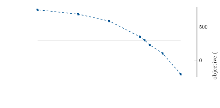
hf_fx.hedging.Without skew the inventory is a random walk and the best policy hedges 95% of every trade. With a half-life of about 1 150 trades or more it still hedges 95%; at 870, 80%; at 770, half; at 690 or less, almost nothing (Figure 21.2). Once the flow offsets itself fast enough, internalising earns far more than hedging: $588 000 a day at a half-life of 350 trades against $300 000 for hedging everything. The switch is abrupt for a reason worth knowing. Without skew the inventory’s variance grows with the square of the unhedged share , and the objective has its maximum at : 97% here. With the skew, a larger inventory is pulled back harder, and the variance grows only about in proportion to : the objective is then nearly linear in , and its maximum sits at a corner.
21.5 Crosses and emerging markets
Crosses and emerging-market currencies are where internalisation and synthesis matter most: their direct markets are thin, their legs through the dollar are liquid, and a provider with flow in many pairs can offset one client’s euro-yen against another’s euro-dollar and a third’s dollar-yen. Non-deliverable forwards (One Quant Book 2, chapter 18) extend electronic making to currencies with capital controls; they settle in dollars on a fixing, so the provider’s risk runs to the fixing date and its hedge is another non-deliverable forward or the onshore market where it has access.
21.6 Strategy files
Strategy file 21.1 — Primary-venue FX market making
Who pays you, and why. Banks and funds that take liquidity on the interdealer venues.
Instruments and venues. Major pairs on the primary interdealer venues.
Signal. A consolidated fair price from all venues, weighted by noise and staleness.
Sizing and execution. Quote at the touch with inventory skew; firm quotes, no last look.
Costs. Venue fees; adverse selection from faster takers.
How it dies. Speed: algorithmic takers remove the arbitrage opportunities and impose adverse selection on slower providers.
Horizon, capacity, infrastructure. Microseconds to seconds; co-location at each venue.
Backtest honestly. Each venue’s data at its own delay; queue positions.
Sources. Chaboud, Chiquoine, Hjalmarsson and Vega (2014).
Strategy file 21.2 — Disclosed streaming to aggregators with last look
Who pays you, and why. Clients who value a streamed price in their own aggregator, by tier.
Instruments and venues. Streams to banks, brokers, platforms and corporates.
Signal. The fair price; each tier’s measured toxicity.
Sizing and execution. Price each tier to its mark-outs; apply last look only where it pays (the toxic tier in the model).
Costs. Rejects that clients remember; the hedge.
How it dies. Clients who move flow to firm liquidity; the Code’s principles on last look and its disclosure.
Horizon, capacity, infrastructure. Milliseconds; hundreds of streams.
Backtest honestly. Rejections as the clients saw them, and the flow lost because of them.
Sources. One Quant Book 2, chapter 15; this chapter.
Strategy file 21.3 — Cross-rate synthesis quoting
Who pays you, and why. Clients trading crosses whose direct markets are thin.
Instruments and venues. A cross and its two legs through a common currency.
Signal. The synthetic cross from the legs’ bids and offers.
Sizing and execution. Quote the cross inside its synthetic width when flow can be internalised; hedge in the legs or the direct market, whichever is cheaper.
Costs. Two legs’ spreads when hedging (2.6 pips on the example).
How it dies. One-sided cross flow that cannot be internalised.
Horizon, capacity, infrastructure. Seconds; data on both legs and the direct cross.
Backtest honestly. Leg prices executable at the cross trade’s time.
Sources. This chapter.
Strategy file 21.4 — Non-deliverable forward electronic making
Who pays you, and why. Investors and companies hedging currencies they cannot deliver.
Instruments and venues. Non-deliverable forwards on electronic platforms.
Signal. Onshore rates where observable, the fixing’s history, related liquid currencies.
Sizing and execution. Quote tiered streams; internalise across tenors and clients; hedge the residual in other forwards.
Costs. Wide hedging markets; fixing risk.
How it dies. Capital-control changes and fixing disputes.
Horizon, capacity, infrastructure. Days to months to the fixing.
Backtest honestly. The fixing as published, with its source’s history.
Sources. One Quant Book 2, chapter 18.
21.7 Tutorial: a hundred prices at once
Goal. Build a consolidated fair price, stream it to three tiers with and without last look, and decide how much of the flow to internalise. End state: the table and Figure 21.2.
The fair price: inverse-variance weights with staleness.
def fair_price(mids, noise_bp, ages_ms, sigma: float) -> tuple[float, np.ndarray]:
    mids, noise_bp, ages_ms = (np.asarray(x, float) for x in (mids, noise_bp, ages_ms))
    var = noise_bp ** 2 + sigma ** 2 * ages_ms
    w = (1.0 / var) / np.sum(1.0 / var)
    return float(w @ mids), w
Listing 21.1. Each venue’s noise plus the rate’s variance since its last update. code/firm/fxlp/firm_fxlp.py The streams on Book 2’s
firm.lastlook.def stream(tiers: dict, hold: float = 5.0, threshold: float = 0.1, policy: str = "asymmetric", sigma: float = 0.05, n: int = 20000, seed: int = 1) -> dict: """tiers: name -> (half-spread bp, share of requests, informed share, informed edge bp). Capture per request is the fill ratio times the mark-out (bp).""" out, tot_req, tot_cap, tot_fill = {}, 0.0, 0.0, 0.0 for i, (name, (half, share, inf, edge)) in enumerate(tiers.items()): reqs = ll.simulate(n, sigma, hold, threshold, policy, inf, edge, seed=seed + i) t = ll.tca(reqs, half) cap = t["fill_ratio"] * t["markout"] out[name] = {**t, "capture": cap, "reject": 1.0 - t["fill_ratio"]} tot_req += share tot_cap += share * cap tot_fill += share * t["fill_ratio"] out["all"] = {"capture": tot_cap / tot_req, "reject": 1.0 - tot_fill / tot_req} return outListing 21.2. Each tier’s requests, the last-look check and its transaction-cost analysis, weighted by the tier’s share. code/firm/fxlp/firm_fxlp.py Internalise or hedge with a skew that brings offsetting flow.
    rng = np.random.default_rng(seed)
    u = rng.random(trades)
    inv = np.empty(trades)
    q = 0.0
    for i in range(trades):
        p_reduce = min(max(0.5 + skew * abs(q), 0.0), 0.95)
        reduce = u[i] < p_reduce
        direction = -math.copysign(1.0, q) if q != 0 else (1.0 if u[i] < 0.5 else -1.0)
        client = direction if reduce else -direction            # our inventory change
        q += client * size * (1.0 - h)
        inv[i] = q
    dP = rng.standard_normal(trades) * sigma_day / math.sqrt(trades)
    spread = trades * size * half_bp
    hedge = trades * size * h * hedge_bp
    var = float(np.sum(inv[:-1] ** 2) * sigma_day ** 2 / trades)          # expected variance of the inventory P&L
    return {"spread": spread, "hedge": hedge, "risk_sd": math.sqrt(var), "realised_inv": float(inv[:-1] @ dP[1:]),
            "objective": spread - hedge - lam * var, "end_inventory": float(inv[-1]),
            "mean_abs_inventory": float(np.mean(np.abs(inv)))}
Listing 21.3. The inventory under a hedge share and a skew; spread, hedge cost and the risk charge. code/firm/fxlp/firm_fxlp.py - Sweep the hedge share for each skew (
hf_fx.hedging).
What to change next. Let informed clients cluster in time; add a second pair and internalise across them; run the streams on firm.exchsim’s venues with their own latencies.
21.8 Build: the FX liquidity provider
Purpose. Price FX from many venues, stream tiered prices with or without last look, and decide internalisation.
Interface. fair_price(mids, noise_bp, ages_ms, sigma), venue_errors, stream(tiers, hold, threshold, policy, sigma, n, seed), internalise(h, seed, trades, size, sigma_day, half_bp, hedge_bp, lam, skew), best_hedge_share, synthetic_cross. Built on firm.lastlook (Book 2).
Rules. Basis points of the rate; milliseconds; amounts in basis points times millions.
Acceptance tests. code/firm/fxlp/tests/: weights by hand and a fresh, precise venue dominating; the consolidated price beats the primary; no rejects without last look, all informed rejected with the asymmetric check; hedging everything leaves no inventory risk; a stronger skew lowers the inventory; the synthetic cross by hand, direct and inverted.
Stretch. Clustered informed flow; several pairs internalised together; streams on firm.exchsim.
Sources and further reading
- A. P. Chaboud, B. Chiquoine, E. Hjalmarsson, C. Vega, Rise of the machines: algorithmic trading in the foreign exchange market, Journal of Finance 69(5), 2014, 2045–2084.
- Bank for International Settlements, Triennial Central Bank Survey, preliminary results, press release, 30 September 2025.
21.9 Exercises
Exercise 21.1 ★
Two venues show 1.08500 and 1.08503 with noise of 0.3 and 0.6 basis point, both fresh. What is the fair price?
Solution
Solution of Exercise 21.1.
Weights and , normalised to 0.8 and 0.2: .
Exercise 21.2 ★
Build euro-yen from euro-dollar 1.0850/1.0851 and dollar-yen 150.20/150.21. How wide is it in pips?
Solution
Solution of Exercise 21.2.
Bid , offer : 2.6 pips (of 0.01 yen).
Exercise 21.3 ★
At 0.4 basis point on $20 billion a day, what does the stream earn before hedging? What does hedging everything at 0.25 cost?
Solution
Solution of Exercise 21.3.
; hedging all at 0.25 basis point costs $500 000.
Exercise 21.4 ★★
Why does last look raise the toxic tier’s capture and lower the others’?
Solution
Solution of Exercise 21.4.
The check rejects every informed request (their move exceeds the threshold) and a share of uninformed ones whose price happened to move for the client. On the toxic tier the informed losses avoided exceed the good trades lost; on the others, with few or no informed requests, only the good trades are lost.
Exercise 21.5 ★★
Why is the best hedge share almost always either near 0 or near 95%?
Solution
Solution of Exercise 21.5.
Without skew the variance is quadratic in the unhedged share and the optimum is 97%; with the skew the variance is about linear in it, so the objective is linear and the optimum is a corner: hedge nearly all or nothing.
Exercise 21.6 ★★
What did Chaboud and co-authors find about who removed triangular arbitrage?
Solution
Solution of Exercise 21.6.
The reduction in triangular arbitrage opportunities came primarily from computers taking liquidity; the reduction in return autocorrelation, from computers providing it.
Exercise 21.7 ★★★
Coding. Rerun firm.fxlp.stream with a hold of 20 milliseconds instead of 5. What happens to the rejects of uninformed tier-3 clients?
Solution
Solution of Exercise 21.7.
Uninformed tier-3 rejects rise from 18.3% to 32.6%: over a longer hold, prices move beyond the threshold more often.
Exercise 21.8 ★★★
Find the flaw. “Our internalisation rate is 90%, so our hedging costs are a tenth of our competitors’; we are the cheapest provider.”
Solution
Solution of Exercise 21.8.
Internalisation pays only if the inventory it holds is offset quickly; a high rate may mean the provider is carrying risk it should hedge (or that its skew is too aggressive for its clients). The comparison must include the inventory’s risk and the skew’s cost in worse prices to clients.
21.10 Problem: A Hundred Prices at Once
Problem 21.1
Weekend problem — a hundred prices at once
A non-bank liquidity provider prices euro-dollar from three venues, streams it to three tiers, and decides what to hedge.
Part I — The market.
- Summarise the dated box.
- What did Chaboud and co-authors find about algorithmic trading in FX?
- How is the fair price built, and how much better is it than the primary?
- Define a synthetic cross and give the example’s width.
Part II — Streams.
- Describe the tiers and the last-look check.
- Give capture and rejects without last look and with the asymmetric check, per tier.
- Why is the symmetric check worse for the provider?
- What does last look cost the clients?
Part III — Inventory.
- Describe the internalisation model and the skew.
- Give the best hedge share at half-lives of 1 150, 870, 770 and 690 trades.
- What does internalising earn at a half-life of 350 trades?
- Why is the switch abrupt?
Part IV — The verdict.
- State the named result: the liquidity provider’s capture and reject rate with and without last look, and the hedge share at which internalising stops paying.
- Which tiers would you give last look, and which firm prices?
- How would you measure the inventory’s half-life in real flow?
- What makes crosses and emerging markets different?
- Which strategy file is most exposed to regulation?
- What does a provider with flow in many pairs gain?
- How would clustered informed flow change the answers?
- In one sentence: what does an FX liquidity provider sell?
Solution
Solution of Problem 21.1.
- $9.6 trillion a day in April 2025; swaps $4 trillion; spot up 42% to 31% of turnover; the dollar on 89% of trades.
- Algorithmic trading improved price efficiency; takers removed triangular arbitrage, providers reduced autocorrelation.
- Inverse-variance weights with staleness; 0.26 against 0.30 basis point.
- See Definition 21.1; 2.6 pips.
- Three tiers at 0.3, 0.5 and 1.0 basis point with 30%, 10% and no informed requests; 5 ms hold; 0.1 basis point threshold.
- Tier 1: 0.125 to 0.200 with 43.5% rejects; tier 2: 0.453 to 0.395 (26.5%); tier 3: 1.008 to 0.851 (18.3%); all: 0.400 to 0.389 (33.4%).
- It also rejects moves in the provider’s favour: 0.282 basis point and 48.8% rejects over all tiers.
- Rejections, the delay, and the information the provider gains from the rejected requests.
- 20 000 trades of $1 million; a share hedged at 0.25 basis point; the skew raises the probability of a reducing trade with the inventory.
- 95%, 80%, 50% and 5%.
- $588 000 a day against $300 000 hedging everything.
- With the skew the variance is about linear in the unhedged share, so the objective is nearly linear.
- Capture 0.400 basis point a request without last look and 0.389 with it, 33% rejected (0.125 to 0.200 on the toxic tier); internalising stops paying when the inventory’s half-life exceeds about 900 client trades, and above about 1 150 the best policy hedges 95%.
- Last look for the toxic tier only; firm prices for the others.
- From the decay of the inventory after large trades, with and without skew.
- Thin direct markets, liquid legs: synthesis and internalisation across pairs.
- Disclosed streaming with last look.
- Natural offsets across pairs and clients, shortening the half-life.
- Informed flow arriving together would make inventories one-sided, lengthening the half-life and favouring hedging.
- Immediacy in a currency, priced by tier, hedged or offset.
21.11 Interview questions
Interview question 21.1 ★ trader
A client lifts your euro-dollar offer for $50 million. Hedge now or wait? What do you look at?
Solution
Solution of Interview question 21.1.
The client’s tier and history, the inventory already held, how fast the flow usually offsets, the primary venue’s depth, and the market’s volatility; hedge the part that the offsetting flow will not absorb.
What the interviewer is looking for: internalisation versus hedging with inputs.
Interview question 21.2 ★★ researcher
How would you measure each client’s toxicity, and what would you do with the measure?
Solution
Solution of Interview question 21.2.
Mark-outs of each client’s fills at several horizons, by client and size; use them to tier, price and choose last-look treatment.
What the interviewer is looking for: mark-outs to tiering.
Interview question 21.3 ★★ developer
Design a system that streams 200 tiered prices on 30 pairs and updates them within 50 microseconds of a venue tick.
Solution
Solution of Interview question 21.3.
One fair-price engine per pair, tier pricing as offsets from it computed incrementally, stream publishers per client connection, all fed from the same market-data path with timestamps.
What the interviewer is looking for: shared fair price, incremental tiers.
Interview question 21.4 ★★ risk
Your internalisation rate rose from 70% to 95% in a month. What could explain it, and what could go wrong?
Solution
Solution of Interview question 21.4.
Flow may have become more two-sided (good), or the skew more aggressive, or hedging thresholds looser (risk); check inventory sizes and their decay, and the P&L of the internalised positions.
What the interviewer is looking for: rate versus risk.
Interview question 21.5 ★★ trader
Explain why a symmetric last-look check is fairer to clients than an asymmetric one, and what it costs the provider.
Solution
Solution of Interview question 21.5.
It rejects moves in either direction, so clients are not rejected only when the price has moved in their favour; the provider also gives up the trades that moved in its favour, lowering its capture (0.282 against 0.389 in the model).
What the interviewer is looking for: symmetry and its price.
Interview question 21.6 ★★★ researcher
With spread , hedging cost and a risk charge , find the optimal hedge share when and when .
Solution
Solution of Interview question 21.6.
Quadratic: , , interior when . Linear: the derivative is constant, so if and otherwise.
What the interviewer is looking for: interior versus corner.