Networks, Hardware and Trading Infrastructure · Technology
13Long-Haul Fibre
In August 2010 a new fibre route between Chicago and New Jersey went into service: shorter than the routes before it, with lower-latency equipment, and quoted at one way between the Cermak building in Chicago and Nasdaq’s data centre in Carteret, some round trip. Its cost was publicly estimated at about 300 million dollars. Before it, prices in New Jersey had responded to Chicago within 7.25 to ; around its opening, the response times drop by 1 to . Within two years microwave networks estimated at 4.2 to had beaten it, and the cable’s buyers had learnt what chapter 10’s floors say: glass is slower than air by 46%, and no amount of digging changes that.
Fibre did not lose. It carries everything that is not the fastest few messages: market data by the gigabit, orders when the weather closes the radio links (chapter 14), the transatlantic routes that no tower can cross, and every connection from a firm’s cabinet to its carrier. This chapter takes a long-haul route apart: the glass and what happens to light in it, the path and how straight it is, the equipment, the subsea cables, the ways of buying fibre, and the new glass that is nearly as fast as air.
13.1 Light in glass: attenuation, amplifiers and dispersion
Standard single-mode fibre at loses about per kilometre (Corning’s datasheet for its ultra-low-loss fibre gives 0.16 typical, 0.17 maximum), so a signal loses half its power every 19 kilometres and a thousandth of it every 190. Over the of glass that the 2010 route must contain (below), the loss would be : no receiver hears that. Long-haul fibre is therefore cut into spans, with an amplifier at the end of each.
Definition 13.1 (Optical amplifier)
An optical amplifier restores the power of the light in a fibre without converting it to an electrical signal, typically by passing it through a few metres of fibre doped with a rare earth and pumped by a laser; placed at the end of each span, it lets a signal cross thousands of kilometres of glass.
The amplifier costs little time (the doped fibre is metres, the pass-through a fraction of a microsecond), which is why the route model below charges per span, an assumption, and why amplification is not the latency problem. Dispersion is.
Definition 13.2 (Chromatic dispersion, dispersion compensation)
Chromatic dispersion is the spreading of a light pulse in a fibre because its different wavelengths travel at slightly different speeds, measured in picoseconds of spread per nanometre of spectral width per kilometre. Dispersion compensation undoes it, either optically, with a length of fibre of opposite dispersion (dispersion-compensating fibre) in each span, or electronically, by signal processing in a coherent receiver.
The same datasheet bounds dispersion at per nanometre per kilometre at : over 1 359 kilometres, a spread of about per nanometre of spectrum, far more than a bit at ten gigabits (). Compensating it optically adds glass to the path: a spool in every span, which the model sets at a fifth of the span’s length. Compensating it electronically adds processing time at the ends instead, and leaves the path alone.
Definition 13.3 (Forward error correction)
Forward error correction (FEC) adds redundant bits to a transmitted signal so that the receiver can correct errors without asking for a retransmission; its decoder must collect a block (or an interleaved group of blocks) before it can correct it, which adds a delay at the receiving end.
FEC lets a link run with a noisier signal, hence longer spans or higher speeds, at the price of a delay per terminal. Laughlin, Aguirre and Grundfest note the same trade-off in microwave radios, whose latency is “dominated by” FEC buffering and interleaving. For low-latency fibre the choices are therefore the ones the model exposes: short spans or long ones, optical or electronic dispersion compensation, heavy FEC or light.
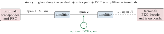
firm.fibreroute charges each piece its time.13.2 Route straightness: the Chicago–New York story
Chapter 10’s floor for 350 Cermak to Carteret is in straight fibre; the 2010 route was quoted at . The difference, , is path and equipment, and inverting the published figure separates them once an equipment time is assumed. With two terminals of and an amplifier every 80 kilometres at (the model’s assumptions, in all), the route must contain 1 359 kilometres of glass: 230 kilometres more than the geodesic, a path factor of 1.20. The later figure of implies 1 339 kilometres, 20 fewer, or faster equipment.
Proposition 13.4 (Inverting a published latency)
If a fibre route of group index is published at one way and its equipment takes , its glass is
and its path factor is for a geodesic . An error in the assumed equipment time moves by , about per microsecond.
Proof. Light covers at in the time left once the equipment’s is removed. Differentiating in gives the sensitivity. ∎
def components(route):
    n = route.spans[0].n_g
    glass = _us(route.geodesic_km, n)
    path = sum(_us(s.km, s.n_g) for s in route.spans) - glass
    dcf = sum(_us(s.dcf_km, s.n_g) for s in route.spans)
    amps = sum(s.amp_us for s in route.spans)
    term = 2 * route.terminal_us
    return {"glass": glass, "path": path, "dcf": dcf, "amps": amps, "terminals": term,
            "total": glass + path + dcf + amps + term}


def invert(published_us, geodesic_km, n_g=1.462, equipment_us=0.0):
    """A published one-way latency, less assumed equipment time, as the glass the route must have."""
    glass_us = published_us - equipment_us
    path_km = glass_us * 1e-6 * C0 / n_g / 1e3
    return {"path_km": path_km, "factor": path_km / geodesic_km,
            "excess_km": path_km - geodesic_km}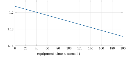
fig_fibre.py, nw_fibre.sensitivity().Figure 13.2 shows why the conclusion is robust: whatever the equipment, most of the millisecond is path. A cable must follow rights of way it can obtain; the 2010 route bought straightness at 300 million dollars and still ran 17 to 20% longer than the geodesic. The microwave networks that beat it had route factors near 1.01 in air (chapter 10) and a medium 46% faster.
| Route | Geodesic | Published | Fibre floor | Glass | Path |
| (km) | (ms, one way) | (ms) | (km) | factor | |
| Chicago–New Jersey, 2010 | 1 129.2 | 6.650 | 5.507 | 1 359 | 1.204 |
| Chicago–New Jersey, later | 1 129.2 | 6.550 | 5.507 | 1 339 | 1.185 |
| New York–London subsea, 2015 | 5 551.0 | 29.475 | 27.070 | 6 038 | 1.088 |
nw_fibre.published().13.3 Subsea cables
Definition 13.5 (Cable landing station)
A cable landing station is the building where a submarine cable comes ashore and connects to terrestrial networks: it powers the cable’s undersea repeaters, terminates its fibre pairs and hands their traffic to land routes.
A subsea route is a terrestrial route at each end, a landing station on each coast, and the ocean between. Hibernia Express, the first new transatlantic cable in over twelve years when it opened in 2015, published a round trip under between Equinix’s NY4 in Secaucus and LD4 in Slough, more than five milliseconds better than the existing cables, over a fibre pair of Corning’s pure-silica-core fibre. The geodesic between the two buildings is ; half the round trip, , implies about 6 040 kilometres of glass, a path factor of 1.09. Across an ocean the geodesic is almost available, apart from the landings and the tails to the data centres; on land, the rights of way cost the Chicago route twice as much in proportion.
Remark 13.6 (Round trips and halves)
Halving a published round trip assumes both directions take the same path and equipment. On a cable pair they usually do; on a network whose two directions ride different fibres or routes they need not, and chapter 4’s asymmetry returns: a round trip cannot tell the two directions apart.
13.4 Dark fibre against leased wavelengths
Definition 13.7 (Dark fibre, lit service, wavelength service)
Dark fibre is fibre sold or leased without equipment: the buyer lights it with its own transponders and amplifiers and controls everything that affects latency. A lit service is capacity sold on the seller’s equipment: a circuit of a given speed between two points. A wavelength service is a lit service that dedicates one wavelength of the seller’s fibre system to the buyer.
Definition 13.8 (Indefeasible right of use)
An indefeasible right of use (IRU) is a long-term contract giving its holder the exclusive right to use specified fibres or capacity of a network for a fixed term, usually paid up front, without transferring ownership of the cable, and usually with a share of maintenance charged to the holder.
An internet carrier’s annual report shows the form in practice: most of its dark fibre is held “in the form of long-term leases under indefeasible rights of use”, it relies on the fibre’s owner to maintain it, and it amortises the IRUs over generally 15 to 20 years. For a trading firm, the choice between dark fibre and a lit service is a choice between control and cost. Dark fibre lets the firm choose its own equipment (light FEC, electronic dispersion compensation, no switches in the path) and costs an IRU, the equipment and yearly maintenance; a lit service costs a monthly fee and gives the seller’s latency.
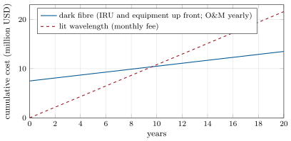
fig_fibre.py, nw_fibre.costs().The break-even arithmetic is simple and its inputs are not: IRU prices and lit fees are negotiated, not published, which is why the figure uses illustrative numbers. With them, dark fibre costs 0.675 million a year spread over twenty years against 1.08 million for the lease, and pays back its up-front outlay after 9.6 years. A firm that expects to keep the route for less than that, or whose strategy may move to microwave, leases; a firm that needs to control every microsecond of the path buys, whatever the break-even says.
def dark(iru, years, om_year, capex, capex_years):
    """Annual cost of dark fibre: the IRU over its term, O&M, and the firm's own
    optical equipment over its life."""
    return iru / years + om_year + capex / capex_years


def lit(monthly):
    return 12 * monthly


def break_even_years(iru, om_year, capex, monthly):
    """Years after which dark fibre (IRU and equipment up front, O&M yearly) has cost less
    in total than a lit service at `monthly`; infinite if the lease is always cheaper."""
    saving = 12 * monthly - om_year
return float("inf") if saving <= 0 else (iru + capex) / saving13.5 Faster glass: hollow-core fibre
Definition 13.9 (Hollow-core fibre)
A hollow-core fibre guides light in a core of air (or vacuum), held by a microstructure of thin glass membranes around it, so that light travels at nearly instead of at .
For decades hollow-core fibre was faster and useless: it lost too much light to cover long distances. A 2025 paper from Microsoft’s fibre team and the University of Southampton reports a hollow-core fibre with a loss of per kilometre at , below the of the best solid silica fibre, with transmission speeds 50% higher, “a 30% reduced latency” and six times less chromatic dispersion than standard telecom fibre. If the loss holds in cabled routes, the fibre floor moves to nearly the air floor.
Figure 13.4 rebuilds the 2010 route four ways with the model (a group index of 1.003 for the hollow core is an assumption consistent with the paper’s 30%). As inverted it takes . With a dispersion-compensating spool of a fifth of each span, it would take : optical compensation costs more than a millisecond on this route, every reason for a low-latency route to compensate electronically. In hollow-core fibre on the same path it would take , less; in standard fibre along the geodesic, . The new glass would save more than any straightening could.
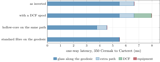
firm.fibreroute: as inverted from its quoted latency, with optical dispersion compensation, in hollow-core fibre on the same path, and in standard fibre along the geodesic. Equipment times, the DCF length and the hollow-core index are the model’s assumptions. Data: fig_fibre.py, nw_fibre.variants().Method 13.10 (Choosing a long-haul fibre route)
- Compute the floor between the two buildings (chapter 10) and ask every seller for a one-way, rack-to-rack latency, with how it was measured.
- Invert each figure into a path factor with a stated equipment assumption; a factor far above the others means a long path or heavy equipment, and the seller should say which.
- Ask how dispersion is compensated and what FEC is used; ask for route diversity (chapter 15) if the route is to carry more than one strategy’s traffic.
- Price dark fibre against a lit service over the expected life of the strategy, not of the fibre.
- Measure the route before and after you depend on it (chapters 4 and 5).
13.6 Tutorial: taking a route apart
Goal. Model a long-haul route as spans, invert published latencies, and see what dispersion compensation and hollow-core fibre change. End state: Figures 13.2, 13.3 and 13.4 and Table 13.1.
- The published figures.
nw_fibre.PUBLISHEDholds each route’s end points and its one-way figure, from the ledger;published()inverts them (Listing 13.1) with the equipment ofEQUIP. - Sensitivity.
sensitivity()repeats the inversion for equipment times from 0 to . - Variants.
variants()rebuilds the route withfirm_fibreroute.buildandwith_index. - Costs.
costs()andbreak_even_years(Listing 13.2) compare buying and leasing with the illustrativePRICES.
What to change next. Replace the equipment assumptions with a seller’s documented figures; add a terrestrial tail to each end of the Atlantic route and see how much of its excess the tails explain.
13.7 Build: the fibre route model
Purpose. Long-haul fibre routes as data and arithmetic: their latency by component, what a published figure implies, and what buying or leasing them costs; used by chapters 14 (the fibre back-up of a radio route), 15 (buying) and 29 (the plan).
Interface. firm_fibreroute: Span(km, n_g, amp_us, dcf_km), Route(name, geodesic_km, spans, terminal_us), build, components, invert, with_index, dark, lit, break_even_years.
Rules. A path is never shorter than its geodesic; every equipment time is a stated parameter; published latencies are one-way and say how they were derived.
Acceptance tests. code/firm/fibreroute/tests/: components by hand, inversion round trip, the hollow-core ratio, a DCF spool, and the break-even arithmetic, including a lease that is always cheaper.
Stretch. Routes as polylines over firm.geomap coordinates; loss and amplifier placement from attenuation.
Sources and further reading
- G. Laughlin, A. Aguirre and J. Grundfest, “Information transmission between financial markets in Chicago and New York”, Financial Review 49(2) (2014).
- M. Petrovich, E. Numkam Fokoua et al., “Broadband optical fibre with an attenuation lower than 0.1 decibel per kilometre”, Nature Photonics (2025).
- Corning, SMF-28 ULL product information (2020); Equinix, release on Hibernia Express (3 November 2015); Cogent Communications, Form 10-K for 2022.
13.8 Exercises
Exercise 13.1 ★
At per kilometre, what fraction of the light is left after an 80-kilometre span?
Solution
Solution of Exercise 13.1.
, a factor : about 5.2% of the light is left.
Exercise 13.2 ★
Using Proposition 13.4, how much glass does a route published at contain if its equipment takes ?
Solution
Solution of Exercise 13.2.
of glass, a path factor of 1.185 over the geodesic.
Exercise 13.3 ★
What is the difference between dark fibre and a wavelength service, from the point of view of latency?
Solution
Solution of Exercise 13.3.
With dark fibre the buyer chooses and controls the equipment (transponders, FEC, dispersion compensation, no switches), so it controls every microsecond beyond the glass; with a wavelength service the seller’s equipment and its choices set the latency, and may change when the seller upgrades.
Exercise 13.4 ★★
Why does optical dispersion compensation cost latency, and electronic compensation not (or much less)?
Solution
Solution of Exercise 13.4.
Optical compensation adds a length of dispersion-compensating fibre to every span, and light takes time to cross it: in the model a fifth of the path, more than a millisecond on the Chicago route. Electronic compensation undoes the dispersion by computation in the receiver, which costs a processing delay at the end of the route, independent of its length.
Exercise 13.5 ★★
The Atlantic route’s path factor is 1.09 and the Chicago route’s 1.20. Give two reasons.
Solution
Solution of Exercise 13.5.
Across the ocean a cable can lie close to the geodesic, with detours only at the landings and the tails to the data centres; on land the route must follow the rights of way it can obtain (roads, railways, utility corridors) around terrain and property. The Atlantic route is also five times longer, so fixed detours at its ends weigh less in proportion.
Exercise 13.6 ★★
A seller quotes a round trip. What must you ask before halving it?
Solution
Solution of Exercise 13.6.
Whether both directions use the same fibres, path and equipment (otherwise the halves differ, and a round trip cannot tell them apart), whether it is rack to rack or between the seller’s own equipment, and whether it is a typical, a best or a guaranteed figure.
Exercise 13.7 ★★★
Coding. With firm.fibreroute, find the path factor at which a hollow-core route between Cermak and Carteret would match a microwave route at a route factor of 1.011 in air.
Solution
Solution of Exercise 13.7.
The microwave route at 1.011 in air takes between the two buildings. Hollow-core glass along the geodesic takes ; with the model’s of equipment the hollow-core path factor must be at most (1.008 without equipment). A hollow-core route would have to be as straight as the microwave route and carry almost no equipment delay.
Exercise 13.8 ★★★
Find the flaw. “Our new fibre route is only 3% longer than the geodesic, so it will beat the microwave networks, whose towers zig-zag.”
Solution
Solution of Exercise 13.8.
A path 3% longer than the geodesic in glass takes times the vacuum floor; a microwave route at a route factor of 1.01 to 1.10 in air takes 1.01 to 1.10 times it. The zig-zag of the towers costs a few per cent; the glass costs 46%. Straightness cannot make up for the medium.
13.9 Problem: Thirteen Milliseconds
Problem 13.1
Weekend problem — taking the 2010 Chicago–New Jersey route apart
The 2010 fibre route from 350 Cermak to Carteret was quoted at one way. Use the model’s assumptions: per terminal, an amplifier every 80 kilometres at , standard fibre of group index 1.462.
Part I — The floor.
- What are the geodesic distance and the floors in vacuum and in fibre between the two buildings?
- What is the round trip quoted, and the round-trip floor in fibre?
- How much of the one-way figure is above the fibre floor?
- Why is the fibre floor, not the vacuum floor, the right comparison for a fibre route?
Part II — The split.
- How much glass does the route contain, and how many spans?
- What is the equipment time in the model, and how much of the excess is equipment?
- How much is extra path, in microseconds and in kilometres?
- What happens to the split if the equipment takes ?
Part III — Other glass.
- What would optical dispersion compensation of a fifth of each span add?
- What would the same path take in hollow-core fibre of group index 1.003?
- And standard fibre along the geodesic?
- How do these compare with the 2016 microwave route of chapter 10 ( from Aurora)?
Part IV — The verdict.
- State the named result: the split of the 2010 round trip into glass along the geodesic, extra path and equipment, and the milliseconds a hollow-core fibre on the same path would save.
- Which part of the split depends most on the model’s assumptions?
- Why did the route lose its lead within two years?
- What did it keep?
- Would you buy it as dark fibre or lease a wavelength on it?
- What would a hollow-core route need to beat the microwave networks?
- What does the Atlantic route’s path factor say about where the Chicago route lost its time?
- In one sentence: where do the thirteen milliseconds go?
Solution
Solution of Problem 13.1.
Part I.
- ; in vacuum, in fibre.
- round trip against a round-trip fibre floor of .
- .
- Because the route is glass: even along the geodesic it cannot beat ; the vacuum floor measures what the medium costs, not what the route wastes.
Part II.
- of glass, in 17 spans of at most .
- (two terminals and 17 amplifiers): 1.9% of the excess.
- of extra path, of glass.
- The path shrinks to , still () more than the geodesic: most of the excess remains path.
Part III.
- : in all.
- , less.
- : straightening would save , hollow core .
- The microwave route reaches Carteret from Aurora, further west, in : faster than hollow core on the 2010 path, faster than the 2010 route.
Part IV.
- Named result: of the round trip, is glass along the geodesic, extra path and equipment (with the model’s assumptions); hollow-core fibre on the same path would save one way, round trip.
- The split between path and equipment: every microsecond of equipment assumed is less path.
- Microwave networks along nearly the same geodesic, in a medium 46% faster, came within 1 to 2% of the air floor.
- Bandwidth and reliability: it carries market data and orders in any weather and backs up the radio links.
- It depends on the strategy’s life and on control: for a firm that must control every piece of equipment for years, dark fibre; for a back-up or a data route, a leased wavelength.
- A path factor within a fraction of a per cent of the geodesic and almost no equipment delay (exercise 13.7).
- That on land the time is lost to the path: the Atlantic cable, with no rights of way to follow, has a factor of 1.09 against the Chicago route’s 1.20.
- Eleven go to light in glass along the geodesic, two to the detours of the path, and almost nothing to the equipment.
13.10 Interview questions
Interview question 13.1 ★ developer
How fast does light travel in fibre, and what is the latency per 1 000 kilometres?
Solution
Solution of Interview question 13.1.
At , about : per kilometre, per one way, against in vacuum or air.
What the interviewer is looking for: The group index; one-way against round trip; the per-kilometre rule of thumb.
Interview question 13.2 ★★ developer
What adds latency to a long-haul fibre route besides the length of the glass?
Solution
Solution of Interview question 13.2.
The path’s detours from the geodesic, optical dispersion compensation (extra glass), amplifiers (small), terminals: transponders and forward error correction, and any switches or routers on the way; plus the tails from the route’s ends to the racks.
What the interviewer is looking for: Path length dominates; DCF against electronic compensation; FEC as a trade of distance against delay.
Interview question 13.3 ★★ developer, trader
Why did microwave beat fibre between Chicago and New Jersey, and why is fibre still used there?
Solution
Solution of Interview question 13.3.
Microwave travels in air at almost , 46% faster than light in glass, along a nearly straight line of towers; fibre follows rights of way and is slower per kilometre. Fibre remains for bandwidth, reliability in bad weather, and everything that is not the few latency-critical messages.
What the interviewer is looking for: Medium and path; capacity and weather; the two used together.
Interview question 13.4 ★★ developer
What is an IRU, and when would a trading firm buy dark fibre rather than lease a wavelength?
Solution
Solution of Interview question 13.4.
A long-term, usually prepaid, exclusive right to use specified fibres or capacity without owning the cable. A firm buys dark fibre when it needs to control the equipment and hence the latency, expects to use the route for longer than the break-even term, and has the staff to run it; otherwise it leases.
What the interviewer is looking for: Control of latency; up-front against monthly cost; maintenance obligations; strategy lifetime.
Interview question 13.5 ★★ developer, researcher
What is hollow-core fibre, and what would it change for latency-sensitive trading?
Solution
Solution of Interview question 13.5.
Fibre that guides light in an air core, so light travels at nearly ; recent designs also lose less light than solid glass. For trading it would cut about 30% from fibre latency, bringing fibre routes close to the air floor with fibre’s bandwidth and weather-independence, and threatening microwave’s advantage on routes that can be built straight.
What the interviewer is looking for: Latency and loss both; the route must still be straight; deployment and cost as open questions.
Interview question 13.6 ★★★ developer
A seller claims a fibre route between two cities that is faster than your computed fibre floor. What could explain it?
Solution
Solution of Interview question 13.6.
The endpoints differ from the ones you computed (a nearer building); the figure is not one-way (a round trip halved over asymmetric paths, or a wrong unit); the route is not all standard fibre (hollow core, or part radio); or the measurement is wrong (unsynchronised clocks). Ask for the endpoints, the method and the medium, and measure.
What the interviewer is looking for: Physics as a sanity check; endpoints and definitions; measurement.