Networks, Hardware and Trading Infrastructure · Technology
14Long-Haul Wireless
When a storm crosses the line of towers between Chicago and New Jersey, the microwave links under it fade, and for as long as the rain lasts the fastest route between the futures and the stocks is fibre again, three milliseconds slower. Shkilko and Sokolov used exactly those afternoons as an experiment: weather episodes that “temporarily remove the speed advantages of the fastest traders by disrupting their microwave networks” were associated with lower adverse selection and lower trading costs. The rain gave the slower traders a few hours without the race, and the market’s liquidity improved while it lasted.
Chapter 10 measured the routes against their floors and chapter 13 took the glass apart. This chapter does the same for the air: the geometry of a line-of-sight hop, the power it has to spare, the rain that takes it away, the millimetre-wave and laser links inside a metropolitan area, the shortwave radio that crosses oceans, and what these links can carry. Its model runs a labelled storm across a chain of towers between Aurora and Carteret and counts the minutes on fibre.
14.1 Microwave links: line of sight, Fresnel zones and towers
Definition 14.1 (Microwave link, line-of-sight path)
A microwave link carries data by radio at frequencies of a few to a few tens of gigahertz between two directional antennas, typically on towers or rooftops. It needs a line-of-sight path: a straight path between the antennas clear of the ground and of obstacles, since such waves do not bend around them.
Definition 14.2 (Fresnel zone, earth bulge)
The first Fresnel zone of a radio path is the ellipsoid around the straight line between the antennas in which paths are at most half a wavelength longer than the direct one; obstacles inside it weaken the received signal, so a link is designed to keep it clear. The earth bulge is the height of the Earth’s surface above the straight line joining two points at ground level, at a given point between them; atmospheric refraction bends radio waves slightly downward, which is modelled by an earth of radius times the real one.
Proposition 14.3 (Hop geometry)
At distances and kilometres from the two ends of a hop of length , the earth bulge is metres and the radius of the first Fresnel zone at gigahertz is metres. At mid-hop, and : the bulge grows with the square of the hop, the zone with its square root.
Proof. A circle of radius rises above its chord, at distances and from its ends, by to first order; with km and the result in metres, . The first Fresnel radius is with ; with in kilometres and in gigahertz the constant is . Setting gives the mid-hop forms. ∎
Laughlin, Aguirre and Grundfest give the same mid-hop rules (8.7 and 1/50) and draw the consequence for the Chicago–New York networks: with towers of about 100 metres, frequencies near , below 4/3 and obstacles of 10 metres, a hop over flat terrain cannot be much longer than about 70 kilometres, so a 1 200-kilometre route needs twenty hops or more. Table 14.1 reproduces the arithmetic.
| Hop | Frequency | Earth bulge | Fresnel radius | Tower height |
| (km) | (GHz) | at mid-hop (m) | at mid-hop (m) | (m) |
| 30 | 6 | 13.2 | 19.4 | 42.6 |
| 30 | 11 | 13.2 | 14.3 | 37.5 |
| 50 | 6 | 36.8 | 25.0 | 71.8 |
| 50 | 11 | 36.8 | 18.5 | 65.3 |
| 70 | 6 | 72.1 | 29.6 | 111.7 |
| 70 | 11 | 72.1 | 21.8 | 104.0 |
nw_wireless.geometry_rows().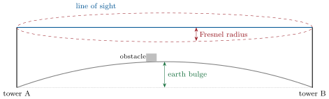
Definition 14.4 (Link budget, fade margin)
A link’s link budget adds the transmitter’s power and the antennas’ gains and subtracts the path’s losses to give the power received. Its fade margin is the received power minus the least power at which the receiver still decodes the signal at the required error rate: the loss the link can absorb before it fails.
The budget follows from physics once the equipment is fixed. Free space loses decibels ( in gigahertz, in kilometres); a dish of diameter gains . With the model’s equipment (30 dBm transmitted, 1.8-metre dishes of 60% efficiency, of other losses, a receiver threshold of dBm, all assumptions), a 60-kilometre hop keeps between 31 and of margin (Table 14.2). Higher frequencies gain more in the dishes than they lose in free space; the rain takes it back.
14.2 Weather, rain fade and availability
Definition 14.5 (Rain fade, link availability)
Rain fade is the attenuation of a radio signal by raindrops along its path, which grows with the rain rate and steeply with frequency. A link’s link availability is the fraction of time in which it carries traffic at its required error rate, usually stated per year.
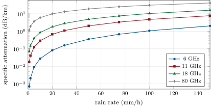
Recommendation ITU-R P.838-3 gives rain’s specific attenuation as a power law of the rain rate, decibels per kilometre for millimetres an hour, with coefficients tabulated by frequency and polarisation. At (horizontal polarisation) and : a storm of costs per kilometre. At , and ; at , and . Figure 14.2 shows the spread: in a light rain of , a factor of about 740 between 6 and .
fig_wireless.py; coefficients in code/firm/radiolink/data/p838_3.csv.Proposition 14.6 (The rain that breaks a hop)
A hop with fade margin decibels fails when rain of rate covers a length of it with , that is above the critical rate
Proof. The rain’s attenuation over the wet length is ; the hop fails when it exceeds the margin. Solving for gives . ∎
A 60-kilometre hop at keeps of margin in the model: rain of along its whole length would break it, but a storm cell ten kilometres across needs . At the same hop survives everywhere; at it fails in a drizzle, which is why long hops use the lower bands and short ones can use the higher.
| Frequency | Dish gain | Free-space loss | Received | Fade margin | , whole hop | , 10-km cell |
| (GHz) | (dBi) | (dB) | (dBm) | (dB) | (mm/h) | (mm/h) |
| 6 | 38.9 | 143.6 | 31.1 | 63.5 | 196.0 | |
| 11 | 44.1 | 148.8 | 36.4 | 18.4 | 80.4 | |
| 18 | 48.4 | 153.1 | 40.7 | 8.1 | 42.3 | |
| 80 | 61.4 | 166.1 | 53.6 | 0.7 | 8.5 |
nw_wireless.budget_rows().def gamma_db_km(rain_mm_h, f_ghz, pol="h"):
k, a = coefficients(f_ghz, pol)
return k * rain_mm_h ** a
def rain_db(hop, rain_mm_h, wet_km=None):
wet = hop.d_km if wet_km is None else min(wet_km, hop.d_km)
return gamma_db_km(rain_mm_h, hop.f_ghz, hop.pol) * wet
def critical_rain(hop, wet_km=None):
k, a = coefficients(hop.f_ghz, hop.pol)
wet = hop.d_km if wet_km is None else min(wet_km, hop.d_km)
fm = fade_margin_db(hop)
return 0.0 if fm <= 0 else (fm / (k * wet)) ** (1 / a)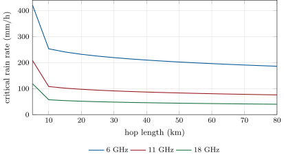
fig_wireless.py, nw_wireless.critical_curve().Availability follows from how often the critical rate is exceeded, which is a property of the climate along the route, published in rain-rate statistics that this chapter does not use. With a labelled model in which it rains 5% of the time with a mean rate of (exponentially distributed), one 59-kilometre hop at soaked end to end is down 0.047% of the year, about four hours; twenty such hops failing independently would put the route on fibre for about 0.9% of the time. The model is crude; the structure is not: availability multiplies along a chain, and a route is only as dry as its wettest hop.
14.3 Millimetre waves and lasers
Definition 14.7 (Millimetre-wave link, free-space optical link)
A millimetre-wave link is a radio link at frequencies of about 30 to 300 GHz (wavelengths of 10 to 1 millimetres), with wide channels and short hops. A free-space optical link (FSO) carries data on a laser beam through the air between two terminals; fog and heavy rain block it, and it needs a clear, stable line of sight.
Inside a metropolitan area the trade-off reverses: hops are short, rain has little path to act on, and bandwidth matters. ICE’s New Jersey routes between Mahwah and Secaucus, run with Anova Financial Networks, combine millimetre-wave and free-space optics over 5-gigabit radio channels; between Mahwah and Carteret they use several 1-gigabit channels. The two technologies fail differently (rain for millimetre waves, fog for lasers), so a route that carries both loses both only when rain and fog come together.
14.4 Shortwave radio across oceans
Definition 14.8 (Skywave propagation)
Skywave propagation carries radio waves of a few to a few tens of megahertz beyond the horizon by reflection from the ionosphere, one or more times, so that a single link can span an ocean.
The geodesic from Secaucus NY4 to Slough LD4 is : of light in vacuum, against in straight glass and for the fastest published subsea route of chapter 13. A single reflection from a layer 300 kilometres high lengthens a 5 551-kilometre path by only about 0.6% in a flat-earth approximation, so a skywave link can beat any cable by about ten milliseconds before its equipment, with a bandwidth far below a microwave channel’s and an availability that follows the ionosphere, hour by hour.
As of September 2026 — Shortwave for trading
Trade press reported in July 2023 that high-frequency traders had used shortwave links for several years to send trading data between U.S. and foreign exchanges under experimental authorisations, and that a Shortwave Modernization Coalition wanted the band opened to fixed, long-distance, non-voice use. The FCC sought comment on the coalition’s petition (RM-11953) by public notice on 30 June 2023.
14.5 Licences, towers, bandwidth and what is sent
A microwave route is public in a way a fibre route is not: in the United States its paths are licensed, and Laughlin, Aguirre and Grundfest used the FCC’s licence records to document at least fifteen Chicago–New York networks, their towers and their lengths. The spectrum is narrow: private networks there use mostly 30- and 40-megahertz channels in the 6- and 11-gigahertz bands, at about 140 to 190 megabits a second per channel in their account. Venue-sold services are narrower still: 1 to 10 megabits of private bandwidth on ICE’s Toronto service, 10 megabits on SIX’s Zurich–Frankfurt network.
What is sent is therefore chosen: the few fields of the few instruments that move another market (an index future’s best price, a trade), in compact formats, with everything else on fibre. The radio’s own latency matters: Laughlin and his co-authors describe radios on the market in 2010 that added tens to thousands of microseconds per hop, mostly in forward error correction and interleaving, and estimate a few to twenty microseconds per hop for the networks then being licensed. A route of twenty hops multiplies each microsecond by twenty.
14.6 A storm across the route
The model runs a storm across the Aurora–Carteret route: twenty hops of on the great circle (), a rain cell across moving across the line at , with its rate falling linearly from a peak at its centre to zero at its edge. While every hop holds its margin, the route runs at the published ; when one fails, it falls back to fibre, which the model takes as a path 20% longer than the geodesic, . Everything but the geometry, the coefficients and the radio route’s published latency is an assumption.
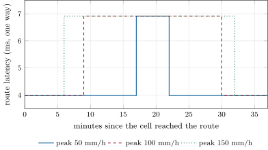
fig_wireless.py, nw_wireless.storm().With a peak of the route spends 21 of the storm’s 38 minutes on fibre, slower; with , 5 minutes; with , 26. The same storms at cost 0, 0 and 7 minutes; at , 22, 29 and 31. For the firms that race, those minutes are the afternoons of Shkilko and Sokolov’s study; for their counterparties, they are when the market is kinder.
def storm_timeline(hops, storm, radio_us, fibre_us):
    """Minute by minute while the cell crosses the route (from one radius before it to one
    after): hops down, and the latency, radio if every hop holds its margin, else fibre."""
    starts = [sum(h.d_km for h in hops[:i]) for i in range(len(hops))]
    out, m = [], 0
    while True:
        y = -storm.radius_km + storm.speed_km_min * m
        if y > storm.radius_km:
            return out
        down = 0
        half = math.sqrt(max(0.0, storm.radius_km ** 2 - y * y))
        for h, s in zip(hops, starts, strict=True):
            lo, hi = max(s, storm.at_km - half), min(s + h.d_km, storm.at_km + half)
            if hi <= lo:
                continue
            dist = math.hypot(y, (lo + hi) / 2 - storm.at_km)
            rate = storm.peak_mm_h * max(0.0, 1 - dist / storm.radius_km)
            if rain_db(h, rate, hi - lo) > fade_margin_db(h):
                down += 1
        out.append((m, down, radio_us if down == 0 else fibre_us))
m += 1Method 14.9 (Evaluating a radio route)
- From the licence records or the provider, get the towers: number of hops, lengths, frequencies. Compute the path’s route factor (chapter 10).
- For each hop, compute the geometry and, with the provider’s equipment figures, the fade margin; find the hops with the least critical rain rate.
- Combine with the climate along the route to estimate availability; ask the provider for its measured availability and its outage history.
- Price the fibre back-up, and design the switch-over: who detects the fade, how fast traffic moves, and what the strategies do meanwhile.
- Decide what the radio carries: the few messages whose speed pays for it.
14.7 Tutorial: a hop, the rain and a storm
Goal. Compute a hop’s geometry and budget, its rain limits by frequency, and a storm’s cost in minutes on fibre. End state: Figures 14.2, 14.3 and 14.4 and Tables 14.1 and 14.2.
- Geometry.
firm_radiolink.bulge_m,fresnel_mandtower_m(Proposition 14.3);nw_wireless.geometry_rows()fills Table 14.1. - Budget.
Hop,rx_dbmandfade_margin_db;budget_rows()fills Table 14.2. - Rain. The P.838-3 coefficients are data (
data/p838_3.csv), each row with its ledger reference;critical_rain(Listing 14.1) implements Proposition 14.6. - The route and the storm.
chainplaces twenty hops on the great circle;storm_timeline(Listing 14.2) runs the cell across one of them.
What to change next. Use vertical polarisation (lower attenuation at these frequencies); shorten the hops to 40 kilometres and add towers; move the storm along the route instead of across it.
14.8 Build: the radio link model
Purpose. Radio hops and chains with their geometry, budget and rain, and the failover to fibre: the air half of the routes that chapters 15, 19 and 29 price and plan.
Interface. firm_radiolink: bulge_m, fresnel_m, tower_m, fspl_db, dish_gain_dbi, Hop, rx_dbm, fade_margin_db, coefficients, gamma_db_km, rain_db, critical_rain, chain, hop_lengths, Storm, storm_timeline, availability.
Rules. Rain coefficients come from the data file with their source, never typed in code; equipment figures are parameters; a storm is a simulation and says so.
Acceptance tests. code/firm/radiolink/tests/: the mid-hop rules, the free-space loss, a budget and the critical rain by hand, the great-circle chain’s end points, a dry and a wet storm, and availability at the extremes.
Stretch. Terrain profiles along each hop; the ITU-R method for the effective path length of rain; correlated rain between neighbouring hops.
Sources and further reading
- A. Shkilko and K. Sokolov, “Every cloud has a silver lining: fast trading, microwave connectivity, and trading costs”, Journal of Finance 75(6) (2020).
- Recommendation ITU-R P.838-3 (2005), specific attenuation model for rain.
- G. Laughlin, A. Aguirre and J. Grundfest (2014), section on microwave networks; ICE, New Jersey metro wireless routes; FCC Order DA 23-689 (2023) and Radio World (July 2023) on shortwave.
14.9 Exercises
Exercise 14.1 ★
What are the earth bulge and the first Fresnel radius at the middle of a 40-kilometre hop at , with ?
Solution
Solution of Exercise 14.1.
Bulge ; Fresnel radius .
Exercise 14.2 ★
What is the specific attenuation of rain at at 6 and at ?
Solution
Solution of Exercise 14.2.
at ; at , twenty times more.
Exercise 14.3 ★
Why can a microwave network have a route factor near 1.01 when a fibre route struggles to get below 1.2?
Solution
Solution of Exercise 14.3.
Towers can be placed almost anywhere a lease can be had, in a nearly straight line, and the signal crosses fields, rivers and roads without needing a right of way along them; a cable must follow continuous corridors in the ground. The route factor measures only the path; the air’s speed is a separate gain of 46%.
Exercise 14.4 ★★
Doubling a hop’s length adds how many decibels of free-space loss, and what does it do to the critical rain rate if the rain covers the whole hop?
Solution
Solution of Exercise 14.4.
more loss, so less margin; and the rain acts over twice the length. In the model a 59-km hop at breaks at of rain along its length; a 118-km hop at .
Exercise 14.5 ★★
Why do metropolitan routes pair millimetre waves with lasers?
Solution
Solution of Exercise 14.5.
Both carry gigabits over the short hops of a city; they fail in different weather (millimetre waves in heavy rain, lasers in fog), so carrying the traffic on both keeps the route up unless both kinds of weather come together.
Exercise 14.6 ★★
A shortwave link crosses the Atlantic ten milliseconds faster than any cable. What can it carry, and what can it not?
Solution
Solution of Exercise 14.6.
It can carry a few compact messages (an index future’s best price, a signal) faster than any cable; it cannot carry a market-data feed, and it is available only when the ionosphere allows, so it needs a cable behind it.
Exercise 14.7 ★★★
Coding. With firm.radiolink, find the peak rain rate at which the model’s storm first puts the route on fibre.
Solution
Solution of Exercise 14.7.
Scanning the peak rate, the first storm that puts the route on fibre has a peak of .
Exercise 14.8 ★★★
Find the flaw. “Our route has twenty hops, each available 99.95% of the year, so the route is available 99.95% of the year.”
Solution
Solution of Exercise 14.8.
Availabilities multiply along a chain: , if the hops fail independently. The route is down about 1% of the year, some 87 hours, twenty times more than one hop; and hops are not independent, since one storm can cover two neighbours, which makes the arithmetic more complicated but does not restore 99.95%.
14.10 Problem: The Storm Between Chicago and New Jersey
Problem 14.1
Weekend problem — what a storm costs a radio route
A firm’s radio route from Aurora to Carteret has twenty hops of about at , runs at one way, and falls back to fibre at . Use the model’s equipment and storm.
Part I — One hop.
- What are the mid-hop earth bulge and Fresnel radius, and the tower height for a 10-metre obstacle?
- What are the hop’s free-space loss, received power and fade margin?
- At what rain rate does it lose its margin if the rain covers the whole hop?
- And if the rain covers ten kilometres of it?
Part II — The storm.
- How long does a cell 30 kilometres across take to cross the route at 48 kilometres an hour?
- With a peak of , how many minutes is the route on fibre?
- How much slower is it during those minutes?
- How does the answer change at 6 and at ?
Part III — The year.
- With the labelled exceedance model, how long is one hop down in a year if the rain covers it end to end?
- What does that give for twenty independent hops?
- Why is the independence assumption doubtful?
- What would shorter hops do?
Part IV — The verdict.
- State the named result: the rain rate at which a 59-kilometre hop at loses its fade margin, and the minutes of fibre-only latency that a storm crossing the route costs.
- What did Shkilko and Sokolov find happens to trading costs during such episodes?
- Why would a firm keep a 6-gigahertz route and an 18-gigahertz one?
- What must the firm’s systems do when the route switches to fibre?
- Which of the model’s inputs would you replace first with real data, and from where?
- What does the storm change for a firm that does not race at all?
- Is the fibre back-up’s latency worth reducing? What would it take (chapter 13)?
- In one sentence: what does the weather do to a latency race?
Solution
Solution of Problem 14.1.
Part I.
- of bulge and of Fresnel radius at mid-hop; towers of .
- of free-space loss, dBm received, of fade margin.
- .
- .
Part II.
- minutes: the model counts 38 one-minute steps.
- 21 minutes.
- one way.
- At the route never leaves the radio; at it spends 29 minutes on fibre.
Part III.
- of the year: about 4.1 hours.
- : about 82 hours a year on fibre.
- Rain is spatially correlated: one storm often covers several neighbouring hops, and a climate’s wet season hits them all; failures cluster in time and space.
- Less free-space loss and a shorter wet length per hop, so each hop tolerates heavier rain; but more towers, more radios and more microseconds of equipment.
Part IV.
- Named result: in the model a 59-kilometre hop at loses its fade margin at of rain along its whole length ( in a ten-kilometre cell); a storm crossing the route puts it on fibre for 21 minutes, slower each way.
- Lower adverse selection and lower trading costs while the fastest traders’ microwave networks were disrupted.
- Diversity against the weather: the lower band survives rain that stops the higher one, which carries more; together they keep more hours on the radio.
- Detect the fade in milliseconds, move the latency-critical traffic to fibre, tell the strategies that their latency assumptions changed (widen, pause or stop the races they can no longer win), and move back when the hop recovers.
- The storm climate along the route (rain-rate statistics) and the provider’s real equipment figures and measured outages.
- Its counterparties are slower for a while: quotes stay up longer and adverse selection falls; it may trade more cheaply.
- Yes if the firm keeps trading during storms; a straighter fibre or hollow-core glass would narrow the gap.
- It switches the fastest traders off for a few minutes or hours, and the market is measurably cheaper while it does.
14.11 Interview questions
Interview question 14.1 ★ developer
Why is microwave faster than fibre between two cities, and what does it cost in exchange?
Solution
Solution of Interview question 14.1.
Radio travels in air at nearly along an almost straight line of towers; light in glass travels at along the ground’s rights of way. The price is bandwidth (tens to hundreds of megabits against terabits), weather (rain fade) and towers to lease and maintain.
What the interviewer is looking for: Medium and path; bandwidth and availability as costs; fibre as back-up.
Interview question 14.2 ★★ developer
What limits the length of a microwave hop?
Solution
Solution of Interview question 14.2.
The Earth’s curvature and obstacles: the towers must lift the line of sight and the first Fresnel zone above the bulge, which grows with the square of the hop; and the link budget: free-space loss and rain take the fade margin away as the hop lengthens.
What the interviewer is looking for: Bulge, Fresnel zone, tower height, link budget; the 70-km order of magnitude.
Interview question 14.3 ★★ developer, trader
It is raining in Pennsylvania. What happens to your Chicago–New Jersey strategy, and what should your systems do?
Solution
Solution of Interview question 14.3.
The radio route may fade; traffic moves to fibre, three milliseconds slower. The systems must detect it, switch, adjust the strategies’ latency assumptions (fewer races, wider quotes, or pauses), and switch back; the firm’s competitors on radio are in the same weather.
What the interviewer is looking for: Detection and switch-over; strategy behaviour; everyone’s radio fades together.
Interview question 14.4 ★★ trader, researcher
How would you use weather-driven outages of microwave networks to study the effect of speed on market quality?
Solution
Solution of Interview question 14.4.
Treat storms along the route as exogenous shocks that remove the fastest traders’ speed advantage; compare liquidity, adverse selection and trading costs in those windows with similar windows without storms, controlling for weather’s other effects; that is Shkilko and Sokolov’s design.
What the interviewer is looking for: Natural experiment; identification; controls for weather affecting demand itself.
Interview question 14.5 ★★ developer
What would you send over a 10-megabit microwave link between two exchanges, and what would you leave on fibre?
Solution
Solution of Interview question 14.5.
The few fields that move the other market (best prices and trades of the leading instruments, or a derived signal), in a compact binary format, and orders if the link carries them; everything else, including full depth and recovery, on fibre.
What the interviewer is looking for: Bandwidth budget; message design; recovery path.
Interview question 14.6 ★★★ developer, researcher
Compare microwave, millimetre-wave, lasers and shortwave for connecting two trading sites 50, 1 000 and 6 000 kilometres apart.
Solution
Solution of Interview question 14.6.
At 50 km: millimetre wave and lasers (gigabits, short hops, weather diversity). At 1 000 km: a microwave chain in the 6–11-gigahertz bands with a fibre back-up. At 6 000 km across an ocean: a subsea cable for everything, and possibly shortwave for a few messages when the ionosphere allows.
What the interviewer is looking for: Distance, bandwidth and weather as the axes; always a fibre back-up.