Networks, Hardware and Trading Infrastructure · Technology
2Switches and Layer-1 Devices
A store-and-forward switch cannot send a 1 518-byte frame on before it has received all of it: at that is of waiting, whatever the switch does afterwards. A layer-1 switch sold to trading firms forwards between its ports in , with less than 100 picoseconds of jitter, and in the words of its data sheet it does “not buffer or queue data”: it never looks at the frame at all. Between the two sit the cut-through switches, which look only at the first bytes. Choosing among them, port by port, is most of what designing the network inside a trading cage means.
This chapter follows a frame through each kind of device, then through the passive devices that let a firm watch its own traffic, and ends with three designs of the same small cage: the latency of each path, the devices each path crosses, and the single devices whose failure would cut a server off.
2.1 Store-and-forward against cut-through
Definition 2.1 (Store-and-forward and cut-through switching)
A switch using store-and-forward switching receives a frame completely, checks its frame check sequence, and only then starts to send it on the output port. A switch using cut-through switching starts to send a frame as soon as it has read the header fields it needs to choose the output port, while the rest of the frame is still arriving.
Proposition 2.2 (What a switch adds)
Let a frame of bytes arrive at on a port whose output is idle and of the same rate, and let be the switch’s internal decision and transfer time. A store-and-forward switch adds to the frame’s latency; a cut-through switch that reads the first bytes adds , independent of the frame’s length. If the output port is busy, or faster than the input (it would run out of bits in the middle of the frame), a cut-through switch must buffer the frame and falls back to store-and-forward for it.
Proof. The last bit leaves the sender at and reaches the far end one serialisation after the first bit left the last device. A store-and-forward switch emits its first bit after its last bit arrived, so the serialisation is paid twice, once into the switch and once out; a cut-through switch emits its first bit after the -th byte arrived, and the two serialisations overlap. If the output is busy the bits must wait; if it is faster than the input it would send faster than the bits arrive, and a frame cannot pause in the middle, so the frame must first be stored. ∎
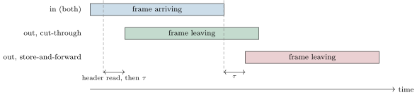
A store-and-forward switch drops a frame whose check sequence is wrong before it goes further; a cut-through switch has already sent most of it when it finds out, and can only mark the end of the frame as bad. That is the whole price of cut-through, and in a colocation cage, where links are short and errors rare, it is a price firms pay.
Example 2.3 (One order, three switches)
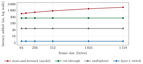
A 100-byte order frame at . A store-and-forward switch with a internal time (a model value, not a data sheet’s) adds ; a cut-through switch that reads 64 bytes adds plus its internal time; a layer-1 device adds only its own few nanoseconds. For a 1 518-byte frame the store-and-forward switch’s toll rises to , the others’ do not change (Figure 2.2).
2.2 Layer-1 devices: fan-out, multiplexing and patching
Definition 2.4 (Layer-1 switch, fan-out, multiplexer)
A layer-1 switch connects ports at the level of the electrical or optical signal: it regenerates the bits of one input on the outputs configured for it without decoding frames, so it neither reads addresses nor queues. A layer-1 fan-out is a configuration that copies one input to several outputs at once. A layer-1 multiplexer merges the frames of several inputs onto one output; unlike a fan-out it must recognise frame boundaries and hold a frame that arrives while another is being sent.
The fan-out is the natural device for market data: the venue’s feed arrives once on the cross-connect and must reach every server that trades on it, all at the same time, with nothing to decide. The multiplexer is the natural device for orders: many servers, one order-entry handoff, and no routing decision beyond “all to that port”. A multiplexer cannot be as fast as a fan-out, because two servers can send at once.
Proposition 2.5 (Contention at a multiplexer)
Two frames of serialisation time reach a multiplexer’s output at times differing by . If the later frame waits ; otherwise neither waits. If each server’s response to a common event arrives with an independent normal delay of standard deviation , is normal with standard deviation and the later of two orders waits with probability .
Proof. The output sends one frame at a time: the frame that arrives second starts when the first has finished, after the first started, or at its own arrival if that is later. The difference of two independent normal variables of variance is normal with variance . ∎
Example 2.6 (Two servers, one handoff)
A 100-byte order occupies of line time at . If two of the firm’s servers answer the same market event with delays of standard deviation , the second order waits with probability . The firm’s own servers are competing with each other at the multiplexer at the moment that matters most, and the one whose response was faster by a few nanoseconds is the one that goes first.
The chapter’s tutorial runs this race for two, four and eight servers (Figure 2.4). With four servers answering within of one another, an order waits on average and the last one , more than the multiplexer’s own ; spread the answers over a microsecond and the average falls to . The tighter a firm’s servers are, the more they queue behind one another.
As of September 2026 — Device latencies from data sheets
Arista’s 7130 Connect Series layer-1 switches forward between ports in ( for the 96-port model), with less than of jitter and the same latency for one-to-many mirroring. Arista’s MetaMux multiplexes several inputs onto one output in on average ( on another hardware model); “when multiple packets arrive at the multiplexer at the same time” it queues them in input buffers, and without contention its latency varies by . Cisco’s Nexus 3548-X cut-through switch quotes latencies “as low as” , in its warp mode, and replicates one port to any number of others in its warp SPAN mode “as low as” .
fig_cage.py.A layer-1 switch is also a patch panel under software control: any port can be connected to any other, or to several, by a configuration change instead of a technician moving a cable. Firms use that to move a server from one venue’s line to another, to swap a failed device for a spare, or to copy a link to a capture device for an hour.
2.3 Taps and mirror ports
A firm that wants to know what it sent and received, and when, must copy its traffic without disturbing it.
Definition 2.7 (Network tap, port mirroring)
A network tap is a device inserted in a link that copies its traffic to monitoring ports; a passive optical tap does it by splitting the light of each fibre, sending a fixed share (its split ratio) to the monitor, needs no power and adds only the length of its fibre. Port mirroring is a switch’s copying of the traffic of some of its ports to another port, in software or in its forwarding hardware.
A tap is on the link itself: it cannot drop, reorder or delay the copy relative to the original, and it keeps working when the switch does not. Its costs are the light it takes (a 50/50 split halves the power reaching the far end, which a long cross-connect may not afford) and a monitoring port for each direction. A mirror port is free, since the switch is already there, but it is a switch port like any other: mirroring both directions of a busy link sends up to to a port, which drops half of it when both directions are full, exactly in the bursts one wanted to see. Capture devices (chapter 5) therefore sit on taps, and on layer-1 mirror outputs, which copy at line rate.
2.4 Designing the network inside one cage
Definition 2.8 (Out-of-band management network, direct-attach cable)
An out-of-band management network is a separate network, with its own switches and links, over which a firm administers its devices and servers, so that configuration, monitoring and remote access never share a port or a queue with trading traffic, and still work when the trading network does not. A direct-attach cable is a copper cable assembly with the transceivers built into its ends, used for short links within a rack.
Method 2.9 (Designing a trading cage’s network)
- List the handoffs: each venue’s market-data lines (A and B), its order-entry connections, and the firm’s own links out.
- Give market data a replication device (a layer-1 fan-out, or a cut-through switch where filtering by group matters), with line A and line B on different devices so that one failure never silences both.
- Give orders a path that crosses as few devices as possible: a layer-1 multiplexer or a cut-through switch per handoff, and a second handoff on a second device.
- Tap every handoff, both directions, and bring the copies to the capture devices; put the time reference (chapter 4) in the same cage.
- Keep management out of band.
- Check the design by removing every device and every cable in turn: each server must still receive at least one line and reach at least one order handoff.
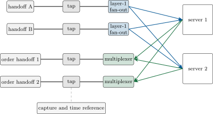
Table 2.1 compares three designs of the same cage, two servers and the same cables (30 metres of cross-connect to each handoff, 3 metres inside the cage), computed with firm.cagenet. The commodity design puts two store-and-forward switches in series; the cut-through design gives each line its own switch; the layer-1 design is Figure 2.3.
| Design | Feed in (ns) | Order out (ns) | Sum (ns) | Single points |
|---|---|---|---|---|
| Store-and-forward switches | 1 439.8 | 1 430.2 | 2 870.0 | both switches, three cables |
| Cut-through switches | 560.0 | 556.8 | 1 116.7 | none |
| Layer-1 devices | 262.8 | 294.6 | 557.3 | none |
nw_cage.design_table() on firm.cagenet.The layer-1 design’s feed path is 263 nanoseconds, of which 176 are the 36 metres of fibre and 83 the frame’s own serialisation: the devices add 4. Its order path is slower than its feed path by the multiplexer’s 39 nanoseconds less the fan-out’s 4, and slower still when two servers answer the same event. The next nanoseconds are no longer in the devices but in the cables and in the servers.
2.5 Tutorial: three cages
Goal. Model a cage’s network, compute its paths and single points of failure, and race orders through a multiplexer. End state: Table 2.1 and Figures 2.2 and 2.4.
- Devices.
nw_cage.DEVICESholds the data-sheet latencies and the one model value;forwarding_curve()evaluates Proposition 2.2 per frame size. - Cages.
design(name)builds each cage fromfirm.cagenetdevices and cables;Cage.pathfinds the route andbreakdownsplits its latency (Listing 2.1). - Failures.
Cage.single_points(feeds, orders, servers)removes each element in turn;design_table()writes the table. - Contention.
mux_contention(k, jitter)races orders through one multiplexer over 20 000 events (Listing 2.2);python fig_cage.pywrites the charts’ data.
What to change next. Replace the cross-connects by 150 metres and see which term of the table dominates; give each server its own multiplexer input from a second network card and measure how contention changes when the firm’s four fastest strategies share two multiplexers instead of one.
    def breakdown(self, path, frame, gbps):
        hops = [self._cable(a, b) for a, b in zip(path, path[1:], strict=False)]
        prop = sum(ns.prop_ns(c.length_m, c.n_g) for c in hops)
        dev = 0.0
        for n in path[1:-1]:
            d = self.dev[n]
            if d.kind in ("l1", "mux"):
                dev += ns.forward_ns(frame, gbps, "layer-1", d.fabric_ns)
            elif d.kind in ("cut-through", "store-and-forward"):
                dev += ns.forward_ns(frame, gbps, d.kind, d.fabric_ns)
return {"serialisation": 8.0 * frame / gbps, "propagation": prop, "devices": dev} rng = np.random.default_rng(seed)
t = np.abs(rng.normal(1000.0, jitter_ns, (n_events, k)))
t.sort(axis=1)
ser = ns.ser_ns(frame, gbps)
free = np.zeros(n_events)
waits = np.zeros((n_events, k))
for j in range(k):
start = np.maximum(t[:, j], free)
waits[:, j] = start - t[:, j]
free = start + ser
return {"mean": float(waits.mean()), "p_wait": float((waits > 0).mean()),
"last": float(waits[:, -1].mean()), "ser": ser}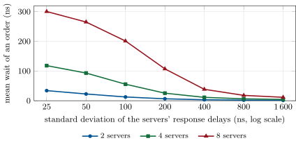
fig_cage.py (seeded).2.6 Build: the cage network model
Purpose. The firm’s cage as data: what is connected to what, with which device, over how much fibre, so that every path’s latency and every single point of failure is computed rather than remembered. Chapter 5 taps it and chapter 29 prices it.
Interface. firm_cagenet: Device(name, kind, fabric_ns) with kinds handoff, server, l1, mux, cut-through, store-and-forward, tap; Cable(a, b, length_m, n_g); Cage(devices, cables) with path, latency_ns, breakdown, single_points(feeds, orders, servers) and untapped(handoffs).
Rules. Latency runs from the first bit at the source to the last bit at the destination; every device’s toll comes from firm.netsim.forward_ns; taps add only fibre; paths never cross a server or a handoff; an unknown device kind or a cable to an unknown device is an error.
Acceptance tests. code/firm/cagenet/tests/: the toll of each device kind on a one-device chain; that a path does not cross a server; single points of failure and untapped handoffs on a hand-built cage.
Stretch. Load: route the feeds of chapter 1 through the cage with firm.netsim.egress at every output and report the worst queue; a spares plan, listing for each single point the patch a layer-1 switch would make to route around it.
Sources and further reading
- Arista, 7130 Connect Series Layer 1 Switch Data Sheet; Arista, 7130 MetaMux product page.
- Cisco, Nexus 3548-X, 3524-X, 3548-XL and 3524-XL Switches Data Sheet.
- Garland Technology, “Network TAP Split Ratios and Loss Budget” (2014).
2.7 Exercises
Exercise 2.1 ★
What does a store-and-forward switch with a internal time add to a 512-byte frame at ? And a cut-through switch reading 64 bytes, with the same internal time?
Solution
Solution of Exercise 2.1.
Store-and-forward: . Cut-through: .
Exercise 2.2 ★
A cut-through switch receives a frame at for an output at , then one at 25 for an output at 10. In which case can it cut through, and why?
Solution
Solution of Exercise 2.2.
From 25 in to 10 out it can cut through: the bits arrive faster than they leave, so the output never runs dry (the difference accumulates in the buffer until the frame ends). From 10 in to 25 out it cannot: the output would send faster than the bits arrive and run out in the middle of the frame, so the frame is stored first.
Exercise 2.3 ★
Both directions of a link are mirrored to one port. The link carries each way at the busiest moment; the mirror port runs at . What share of the copy is lost at that moment?
Solution
Solution of Exercise 2.3.
offered to a port: , about 17% of the copy is lost while both directions are that busy.
Exercise 2.4 ★★
Two servers answer an event with independent normal delays of standard deviation ; their 100-byte orders go through one multiplexer. What is the probability that the later order waits?
Solution
Solution of Exercise 2.4.
has standard deviation ns: .
Exercise 2.5 ★★
In the layer-1 design of Table 2.1, split the feed path’s 262.8 ns into serialisation, fibre and devices. Which would you shorten first, and how?
Solution
Solution of Exercise 2.5.
Serialisation ns, fibre ns, devices 4 ns. The fibre: shorter cables inside the cage and, above all, a shorter cross-connect, which is the venue’s to decide (chapter 9); the serialisation next, by a faster link.
Exercise 2.6 ★★
Why does a fan-out need no buffer while a multiplexer does? What does that imply for their latency and jitter?
Solution
Solution of Exercise 2.6.
A fan-out copies one input to outputs that carry nothing else: an output is never busy when its bits arrive, so nothing waits. A multiplexer’s output is shared by several inputs, and a frame arriving while another is being sent must wait for it. The fan-out’s latency is a constant; the multiplexer’s is a constant plus a queueing delay that depends on the other inputs, its jitter.
Exercise 2.7 ★★★
Coding. Add a third order handoff and a third multiplexer to the layer-1 design, send server 1’s orders through one and server 2’s through the others, and recompute the mean wait of Figure 2.4 for four servers at when the four split two and two across two multiplexers.
Solution
Solution of Exercise 2.7.
Each multiplexer now serves two servers: the mean wait at falls from 93.2 ns (four on one) to 22.7 ns (two on each), the value of mux_contention(2, 50); the design gains a handoff and a multiplexer.
Exercise 2.8 ★★★
Find the flaw. “Line A and line B come into the same layer-1 switch, which fans each out to our servers. It is a single box, but layer-1 switches have no software to crash, so there is no single point of failure.”
Solution
Solution of Exercise 2.8.
One box has one power path, one chassis, one set of optics and one configuration: a power supply or a configuration change takes both lines at once. Put line A and line B on different devices, as the method says; lack of software removes one failure mode, not the others.
2.8 Problem: Three Designs for One Cage
Problem 2.1
Weekend problem — nanoseconds, failures and money
A firm is choosing among the three designs of Table 2.1 for a cage that trades on a signal from the venue’s feed and answers with an order to the same venue. Suppose that the cut-through design costs 60 000 a year more than the commodity design, and the layer-1 design 150 000 a year more (currency units; the figures are the problem’s, not market prices).
Part I — The paths.
- What is each design’s trigger path, from the first bit of the feed frame at the handoff to the last bit of the order at the order handoff, counting feed in and order out?
- How much does the cut-through design save over the commodity one, and the layer-1 design over the cut-through one?
- In the commodity design, how much of the feed path is the two switches’ serialisation?
- How long is the 36 metres of fibre of the layer-1 feed path, in nanoseconds?
Part II — Contention.
- Four of the firm’s strategies share the layer-1 design’s first multiplexer and answer an event within (standard deviation) of each other. What is the mean wait of an order (from the chapter’s simulation)?
- And of the last of the four?
- Does the design still beat the cut-through design for the last order?
- How would you spread the four strategies?
Part III — Failures.
- List the commodity design’s single points of failure.
- Why does the cut-through design have none although each line has only one switch?
- What must be true of the venue’s order handoffs for the layer-1 design to have none?
- What happens to latency when one of the layer-1 design’s fan-outs fails?
Part IV — The verdict.
- What is the cost per nanosecond per year of moving from commodity to cut-through?
- And of moving from cut-through to layer-1?
- State the named result: the trigger path of each design and the cost of each nanosecond saved.
- For which kind of strategy is the layer-1 step worth its price?
- What does a layer-1 design give up that a switch provides?
- Where do the next nanoseconds come from once the devices add only tens?
- Which checks from the method would you run before signing off the design?
- In one sentence: what is the fastest device in a cage?
Solution
Solution of Problem 2.1.
- Commodity ns; cut-through ns; layer-1 ns.
- 1 753.3 ns; then 559.4 ns.
- Two serialisations of the 104-byte frame, ns, plus of the model’s internal time.
- ns.
- 93.2 ns.
- 186.1 ns.
- Yes: ns against the cut-through order path’s 556.8 ns.
- Across the two multiplexers, two each, with the two most correlated strategies on different ones.
- Both switches, the cable between them and the two cables to the servers.
- Each line has its own switch and each switch reaches both servers and its own order handoff: losing one switch loses one line and one order path, never all of either.
- Two order handoffs, each on its own multiplexer, and the venue accepting orders on both (two sessions).
- Nothing for the servers: they take the other line, which has the same latency; the firm loses its protection against the next failure until the device is replaced.
- per nanosecond a year.
- per nanosecond a year.
- Named result. Trigger paths of 2 870, 1 117 and 557 ns; the first 1 753 nanoseconds cost about 34 a year each, the next 559 about 161 each.
- One that wins or loses races decided by hundreds of nanoseconds on this venue, such as the latency-arbitrage and market-making strategies of One Quant Book 11.
- Filtering by address or group, routing between segments, per-port queues and counters of a switch; the design must do its own filtering on the server.
- From the cables (the cross-connect’s length), from serialisation (faster links) and from the servers themselves (chapters 3 and 8, and One Quant Book 13).
- The single-point check, the tap check, and a capture of the real paths against the computed ones (chapter 5).
- One that does not read the frame at all.
2.9 Interview questions
Interview question 2.1 ★ developer
What is the difference between store-and-forward and cut-through switching, and when does a cut-through switch store and forward?
Solution
Solution of Interview question 2.1.
Store-and-forward receives the whole frame, checks it and then sends it: it adds a full serialisation. Cut-through starts sending after the header: it adds a constant. It stores and forwards when the output is busy or faster than the input, and on switches that must rewrite the frame.
What the interviewer is looking for: the serialisation term and the fallback conditions.
Interview question 2.2 ★ developer
What is a layer-1 switch, and what can it not do that an Ethernet switch can?
Solution
Solution of Interview question 2.2.
A device that connects ports at the signal level, regenerating bits without decoding frames: nanoseconds, no queues, fan-out and patching under software control. It cannot read addresses, filter groups, route, or merge traffic from several ports (a multiplexer, which is a different device, does that with a queue).
What the interviewer is looking for: no framing, hence no filtering and no contention.
Interview question 2.3 ★★ developer
Why do firms put orders through a multiplexer rather than a fan-out, and what goes wrong when several servers send at once?
Solution
Solution of Interview question 2.3.
Orders go many to one; a fan-out goes one to many. A multiplexer merges them with a small queue: when several servers answer the same event within a frame’s serialisation, their orders queue behind one another, and a firm’s fastest strategies collide exactly when they matter. Spread correlated strategies over several handoffs.
What the interviewer is looking for: contention that correlates with market events.
Interview question 2.4 ★★ developer
Tap or mirror port for latency measurement? Defend your choice.
Solution
Solution of Interview question 2.4.
A tap: it is on the link, copies every bit including errors at the same time as the original, cannot drop the copy, and keeps working when the switch does not. A mirror port is a switch output that can be oversubscribed and whose copy passes through the switch’s own queueing, so its timing is not the wire’s.
What the interviewer is looking for: oversubscription and timing fidelity of the copy.
Interview question 2.5 ★★★ developer, trader
Design the network for a cage with two venue lines, one order handoff and four servers. Walk me through the failure cases.
Solution
Solution of Interview question 2.5.
Line A and line B through separate taps to separate fan-outs, each fanning out to all four servers; orders from each server through a multiplexer to the handoff, and a second handoff and multiplexer if the venue allows; capture on every tap; management out of band. Failures: a fan-out (servers use the other line), a multiplexer (servers use the second handoff, or stop if there is none: the single point to negotiate away), a cable, a server (its strategies move).
What the interviewer is looking for: no shared device between A and B, and an honest statement of what remains single.
Interview question 2.6 ★★ developer
Your cut-through switch shows higher latency at the open than at noon, for the same frames. Why?
Solution
Solution of Interview question 2.6.
At the open the output ports are busy: frames that find their output sending another frame are stored and wait, so the switch adds queueing (and loses cut-through for those frames). Look at the egress queue occupancy and at microbursts (chapter 1), not at the data sheet’s idle latency.
What the interviewer is looking for: load-dependent queueing and the fallback to store-and-forward.