Networks, Hardware and Trading Infrastructure · Technology
17Where the Crypto Venues Live
Many of the largest crypto venues run their matching engines in or next to a public cloud region rather than in an exchange’s own data centre, and for several of them the cloud provider says so. An AWS blog of June 2026 puts Binance in Tokyo, Bybit in Singapore, Coinbase in the United States and Deribit in London; research reported by CoinDesk in March 2026 puts Hyperliquid’s validators in AWS’s Tokyo region, alongside Binance and KuCoin infrastructure; BitMEX moved its platform from AWS’s Irish region to Tokyo because more than 200 milliseconds separated it from the firms that traded it. A firm that wants to be close launches machines in the venue’s region, measures, and keeps the few that happen to sit nearest the venue’s servers.
Chapter 16 described the cloud; this chapter is about finding a venue in it. What is publicly known about where the venues are; how to find out when it is not published (the provider’s address ranges, the round trips from known places); the lottery of launching machines until one lands close; and the re-measurement that notices when the venue moves. Everything that is not a venue’s or a provider’s own statement is a labelled simulation.
17.1 The publicly known locations
As of September 2026 — Where the cloud-hosted crypto venues are, from public sources
- AWS (June 2026): “Major exchanges operate across Regions: Binance in Tokyo, Bybit in Singapore, Coinbase in the US, and Deribit in London.”
- Glassnode research reported by CoinDesk (March 2026): Hyperliquid’s 24 validators across several availability zones of AWS’s ap-northeast-1 (Tokyo) region, its API behind AWS CloudFront; Hyperliquid, Binance and KuCoin concentrating infrastructure in ap-northeast-1; Tokyo users reaching the validators in 2 to 3 milliseconds, European users in more than 200.
- AWS case study: BitMEX moved its trading platform from the Europe (Ireland) Region to Asia Pacific (Tokyo), with a ten-minute cutover, order execution below 10 milliseconds and liquidity up more than 185% across core contracts.
The box is short because the sources are few. Venues rarely publish their region in their own documentation; the providers mention them in blogs and case studies; researchers infer them from measurements. A region is also only a start: chapter 16 showed that inside it the zone matters by hundreds of microseconds, and the venue’s zone identifier is published even more rarely.
Definition 17.1 (Autonomous system, anycast, edge network)
An autonomous system (AS) is a group of IP prefixes run by one or more network operators under a single routing policy, identified by a number in the internet’s routing system. Anycast is the practice of making one service address available in several places at once, so that each packet reaches whichever is nearest in the routing system. An edge network is a provider’s set of points of presence close to users, often reached by anycast, that terminates connections and forwards requests to the origin servers.
Anycast and edge networks are why looking up a venue’s public address often says nothing about its matching engine. Hyperliquid’s API, in the report above, is reached through the provider’s edge network, while its validators sit in one region; a user in Europe resolves the same name as a user in Tokyo, reaches a nearby edge, and still waits for the round trip to Tokyo behind it.
17.2 How to discover a location
A provider that publishes its address ranges gives the first clue. AWS publishes a file, ip-ranges.json, listing each prefix with its region and the service that uses it. Matching a venue’s endpoint addresses against it by longest prefix says which region an address belongs to, or that it belongs to the edge network, in which case it says nothing about the origin.
def load_ranges(path=DATA / "ip_ranges_fixture.json"):
    with open(path) as f:
        doc = json.load(f)
    out = [(ipaddress.ip_network(p["ip_prefix"]), p["region"], p["service"]) for p in doc["prefixes"]]
    out += [(ipaddress.ip_network(p["ipv6_prefix"]), p["region"], p["service"]) for p in doc.get("ipv6_prefixes", [])]
    return out


def match(ranges, address):
    """Longest-prefix match of an address against the published ranges."""
    ip = ipaddress.ip_address(address)
    hits = [(n, r, s) for n, r, s in ranges if n.version == ip.version and ip in n]
    if not hits:
        return None
    n, r, s = max(hits, key=lambda h: h[0].prefixlen)
return str(n), r, s| Endpoint address | Longest matching prefix | Region | Service |
|---|---|---|---|
| 192.0.2.200 | 192.0.2.128/25 | ap-northeast-1 | EC2 |
| 198.51.100.7 | 198.51.100.0/24 | ap-southeast-1 | EC2 |
| 203.0.113.9 | 203.0.113.0/24 | GLOBAL | CLOUDFRONT |
| 2001:db8:1abc::1 | 2001:db8:1000::/36 | ap-northeast-1 | EC2 |
nw_find.lookups().Definition 17.2 (Round-trip triangulation)
Round-trip triangulation estimates where a server is from round trips measured to it from probes at known places: each round trip bounds the distance (light cannot cover more than half of it in glass) and, divided by a route factor, estimates it; the estimate is the point whose distances best agree with those estimates.
Proposition 17.3 (The light-time bound)
A server that answers a probe in a round trip , of which is equipment and processing on the way, lies within of the probe along the geodesic, for the smallest group index on the path.
Proof. Half the round trip less the equipment is the most time the signal can have spent travelling one way; at speed it covers at most that distance, and no path is shorter than the geodesic. ∎
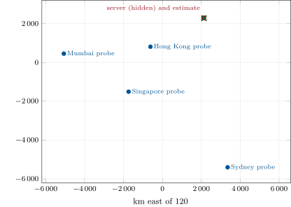
The bound is exact; the estimate is not. In the chapter’s example, probes in Hong Kong, Singapore, Sydney and Mumbai measure round trips of 36.5, 67.4, 98.8 and to a server hidden in Tokyo (a labelled simulation, with paths 30% longer than the geodesics and some noise). Triangulation with the right route factor, 1.3, puts the server within of the truth; with 1.2 or 1.4 it misses by more than . Triangulation from other cities finds the region; inside the region the firm must measure from inside.
fig_find.py, nw_find.triangulate_example().def triangulate(probes, lat0, lon0, span_deg=6.0, step_deg=0.1, n_g=1.462, factor=1.3,
overhead_us=0.0):
"""probes: [(lat, lon, rtt_us)]. A round trip bounds the distance (light in glass) and
estimates it as bound / factor; least squares on a grid around (lat0, lon0)."""
best = None
grid = np.arange(-span_deg, span_deg + 1e-9, step_deg)
for dlat in grid:
for dlon in grid:
lat, lon = lat0 + dlat, lon0 + dlon
res, ok = 0.0, True
for plat, plon, rtt in probes:
d = gm.haversine_m(plat, plon, lat, lon) / 1e3
bound = distance_bound_km(rtt, n_g, overhead_us)
if d > bound:
ok = False
break
res += (d - bound / factor) ** 2
if ok and (best is None or res < best[0]):
best = (res, lat, lon)
if best is None:
raise ValueError("no point satisfies every probe's light-time bound")
return best[1], best[2], math.sqrt(best[0] / len(probes))17.3 The instance lottery
Definition 17.4 (Instance lottery)
The instance lottery is the practice of launching many cloud machines in a venue’s region and zone, measuring each one’s round trip to the venue, keeping the fastest few and releasing the rest, because the provider places each machine without telling the customer where.
Inside one zone, where a new machine lands decides its distance from the venue’s servers: the same rack, the same row, another hall. The provider does not say, so the firm draws. AWS’s blog of June 2026 reports that placement groups, adapter tuning and kernel bypass “can achieve sub-150 µs intra-Region latencies”, and chapter 16’s measurement puts a typical round trip within a zone at . The model takes those two figures as the median and the best 1% of launches, with lognormal round trips between them: an assumption, labelled.
Proposition 17.5 (Best of )
If launches’ round trips are independent draws from a distribution , the expected best of is , which falls with ever more slowly. If each launch costs and each microsecond saved is worth , the best number of launches maximises .
Proof. The minimum of independent draws exceeds only if all do, with probability ; the expectation of a positive variable is the integral of its survival function. The net value is the saving against a single launch less the launches’ cost. ∎
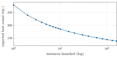
fig_find.py, nw_find.lottery_curve().The curve is the order statistics of Proposition 17.5: one launch expects , ten 185, forty 157, a hundred and sixty . Whether the next launch is worth it depends on what a microsecond is worth. At an assumed 100 USD a month per microsecond and a launch that costs a day of a 16-vCPU instance (17.14 USD at chapter 16’s price), the best is 77 launches, worth about 11 700 USD a month net of their cost (Figure 17.3).
def _draw(lot, size, rng):
    sigma = math.log(lot.median_us / lot.p01_us) / Z
    return lot.median_us * np.exp(rng.normal(0.0, sigma, size))


def expected_best(lot, n, sims=20000, seed=0):
    rng = np.random.default_rng(seed)
    return float(_draw(lot, (sims, n), rng).min(axis=1).mean())


def best_n(lot, value_per_us_month, launch_cost, n_max=200, sims=4000, seed=0):
    """n maximising the monthly value of the round trip saved, net of the launches' cost."""
    base = expected_best(lot, 1, sims, seed)
    best = (1, 0.0)
    for n in range(1, n_max + 1):
        net = value_per_us_month * (base - expected_best(lot, n, sims, seed)) - launch_cost * n
        if net > best[1]:
            best = (n, net)
    return best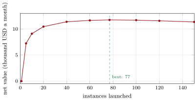
fig_find.py.17.4 Continuous re-measurement
The lottery’s winners do not stay winners. The venue may move within the region or to another region, as BitMEX did; the provider may migrate machines; maintenance may reshuffle a zone. A firm that measured once will notice only when its fills get worse. The chapter’s check is Book 7’s CUSUM test on the daily median round trip from each kept machine: the cumulative sum of standardised recursive residuals, flagged when it leaves its 5% boundary.
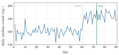
fig_find.py, nw_find.drift_example().The CUSUM test is slow by design: it was built to detect a change in the mean without crying wolf, and here it needs twelve days to be sure of a shift of four standard deviations. A firm that races will add a faster alarm (a jump in the median beyond a fixed threshold, confirmed the next day) and use the CUSUM test to confirm; the lottery then starts again.
Method 17.6 (Finding and following a cloud-hosted venue)
- Read what is public: the venue’s documentation and announcements, the provider’s blogs and case studies, research; record each claim with its source and date.
- Match the venue’s endpoint addresses against the provider’s published ranges; distinguish origin regions from edge networks.
- Triangulate from probes in other regions to confirm the region; inside it, launch machines in every zone and measure.
- Run the lottery in the best zone: launch, measure with hardware timestamps, keep the best, release the rest; stop where the next launch is worth less than it costs.
- Re-measure every day; flag changes; start again when the venue or the provider moves.
17.5 Tutorial: find the venue, win the lottery
Goal. Match addresses, triangulate a server, simulate the lottery and a move, with no cloud account. End state: Figures 17.1, 17.2, 17.3 and 17.4 and Table 17.1.
- Addresses.
firm_venuefind.load_rangesreads the fixture (documented format, documentation addresses);match(Listing 17.1) finds the longest prefix. - Triangulation.
nw_find.probes()simulates round trips from four sites of the site table;triangulate(Listing 17.2) estimates the server. - Lottery.
expected_bestandbest_n(Listing 17.3) withLOTTERY,VALUEandLAUNCH. - Re-measurement.
movedwrapsfirm_decay.cusum.
What to change next. Replace the simulated probes with round trips measured from machines you run; give the lottery a two-tier distribution (same rack or not) and see how the best changes.
17.6 Build: the venue finder
Purpose. Where a cloud-hosted venue is and how close the firm’s machines are to it: the input of chapters 18 and 19 and of the cloud rows of chapter 29’s plan.
Interface. firm_venuefind: load_ranges, match, distance_bound_km, triangulate, Lottery, expected_best, best_n, moved (Book 7’s firm.decay wrapped, not edited).
Rules. Public location claims carry their source and date; an edge address is never taken for an origin; triangulation respects every light-time bound; the lottery’s distribution is a stated assumption until replaced by measurements.
Acceptance tests. code/firm/venuefind/tests/: longest-prefix matching (IPv4 and IPv6), triangulation of a known point and refusal of an impossible one, the lottery’s monotonicity, and the CUSUM flag with and without a move.
Stretch. Probe round trips through the edge to separate its delay from the origin’s; a two-sided change detector tuned for speed.
Sources and further reading
- AWS for Industries blog, “Ultra-low-latency cross-Region crypto trading with Avelacom and AWS” (June 2026); AWS case study on BitMEX; AWS documentation of its IP address ranges.
- CoinDesk, “Hyperliquid traders in Tokyo get 200-millisecond edge, Glassnode research shows” (30 March 2026).
- RFC 1930 (autonomous systems), RFC 4786 (anycast), RFC 5737 and RFC 3849 (documentation address ranges).
17.7 Exercises
Exercise 17.1 ★
A probe measures a round trip of to a server. How far away can the server be, at most, in fibre?
Solution
Solution of Exercise 17.1.
At most along the geodesic, and less once equipment and processing are taken out.
Exercise 17.2 ★
Why does matching a venue’s API address against a provider’s ranges sometimes locate nothing useful?
Solution
Solution of Exercise 17.2.
Because the address may belong to the provider’s edge network (reached by anycast), which terminates connections near the user and forwards them to the origin: the lookup then says “global edge”, not the region of the matching engine.
Exercise 17.3 ★
Using Figure 17.2, how much does the tenth launch save compared with the first, and the hundred-and-sixtieth compared with the fortieth?
Solution
Solution of Exercise 17.3.
The expected best falls from 279 to over the first ten launches, ; from forty to 160 launches it falls from 157 to 138, .
Exercise 17.4 ★★
Why does triangulation from other cities find a region but not a zone?
Solution
Solution of Exercise 17.4.
Zones are kilometres apart, a few microseconds of light, while the uncertainty of a triangulation from thousands of kilometres away (route factors, equipment, noise) is tens or hundreds of kilometres. Inside the region, only machines in each zone measuring the venue directly can tell the zones apart.
Exercise 17.5 ★★
BitMEX moved from Ireland to Tokyo. What changed for a market maker running in Ireland, and what should it have done?
Solution
Solution of Exercise 17.5.
Its round trip to the venue went from within one region to more than across the world: it could no longer quote competitively. It should have followed the venue: read the announcement, launched machines in the new region before the cutover, run the lottery there, and moved its quoting engine.
Exercise 17.6 ★★
Why is the CUSUM test slow, and what would you pair it with?
Solution
Solution of Exercise 17.6.
It accumulates evidence until the path crosses a boundary set for a 5% false-alarm rate over the whole sample, so it waits for many days of evidence; here twelve days for a shift of four standard deviations. Pair it with a fast threshold on the daily or hourly median, confirmed by a second measurement, and keep the CUSUM test to confirm and to catch slow drifts.
Exercise 17.7 ★★★
Coding. With firm.venuefind, find the best number of launches if a microsecond is worth only 20 USD a month.
Solution
Solution of Exercise 17.7.
best_n(LOTTERY, 20.0, 17.14) gives 23 launches, worth about 1 830 USD a month net: the optimum moves down and the prize shrinks by a factor of six.
Exercise 17.8 ★★★
Find the flaw. “Our machine pings the venue’s API in from Frankfurt, so the venue is in Frankfurt.”
Solution
Solution of Exercise 17.8.
The API may be served by an edge network that answers from a point of presence near Frankfurt and forwards to the origin elsewhere; the round trip measures the distance to the edge, not to the matching engine. Measure what the orders actually traverse (the order-entry path, or the time from an order to its acknowledgement), and look at the address against the provider’s ranges.
17.8 Problem: Launch Forty, Keep One
Problem 17.1
Weekend problem — how many machines to launch
A firm trades a venue that runs in one zone of a cloud region. Its launches’ round trips to the venue are lognormal with a median of and a best 1% at . A microsecond is worth 100 USD a month to it; a launch, measured for a day, costs 17.14 USD.
Part I — The draws.
- What is the expected round trip of a single launch?
- And the expected best of 10, 40 and 160?
- Why is the expected single round trip above the median?
- What does Proposition 17.5 say about the shape of the curve?
Part II — The economics.
- What is the net value of keeping the best of 40?
- What number of launches maximises the net value, and what is it worth?
- How flat is the optimum?
- What if a microsecond is worth 20 USD a month?
Part III — Where the draws come from.
- Which facts of chapter 16 and of the AWS blog does the model use, and which assumptions?
- Why may launches not be independent?
- What else than the instance’s position changes its round trip?
- How would you replace the assumption with data?
Part IV — The verdict.
- State the named result: the expected best round trip among instances and the number of launches that maximises value per microsecond net of launch cost.
- How long does the winner stay a winner?
- What does a venue that publishes its zone identifier change?
- Is the lottery fair to the venue’s other users?
- What would a venue do to end it?
- What does the lottery cost a firm that does not race?
- Where does this go in the connectivity plan of chapter 29?
- In one sentence: why launch forty and keep one?
Solution
Solution of Problem 17.1.
Part I.
- (a lognormal’s mean exceeds its median).
- 185, 157 and .
- The lognormal is skewed to the right: rare slow launches pull the mean above the median.
- Each extra launch saves less than the one before: the expected best falls ever more slowly, so the optimum is finite.
Part II.
- About 11 400 USD a month.
- 77 launches, about 11 700 USD a month net.
- Very flat: 40 and 120 launches are within a few per cent of the optimum.
- 23 launches, about 1 830 USD a month.
Part III.
- Facts: the published median round trip within a zone (, chapter 16) and the AWS blog’s “sub-150 µs” intra-Region figure. Assumptions: that they are the median and the best 1% of launches, the lognormal shape, independence, the value and the cost.
- The provider may place successive launches near each other (or deliberately apart), and capacity changes over the day.
- The instance type and its network card, its tuning and kernel-bypass stack, the host’s other tenants, and the venue’s own servers and load balancers.
- Launch, measure each machine’s round trip distribution with hardware timestamps, and fit the distribution; repeat on different days.
Part IV.
- Named result: with the model’s distribution the expected best round trip falls from for one launch to 185 for ten, 157 for forty and 138 for 160; at 100 USD a month per microsecond and 17.14 USD a launch, 77 launches maximise the net value, about 11 700 USD a month.
- Until the venue or the provider moves something: re-measure every day and restart the lottery on a flag.
- The zone: the lottery then runs only inside the right zone, and nobody wastes launches in the others.
- It is open to every user who pays for launches, but it rewards the ones who can afford many; a venue that wants equal access would equalise, as chapter 9’s venues do.
- Offer equal-latency access points (private endpoints in each zone with equal paths, chapter 18), or add a delay that removes the difference.
- Nothing: it launches one machine in the right zone and accepts the median.
- In the cloud rows: the zone, the machines kept, the re-measurement routine and the launch budget.
- Because the provider places machines at random distances from the venue, and the best of forty is worth more than the forty launches cost.
17.9 Interview questions
Interview question 17.1 ★ developer
How would you find out which cloud region a crypto exchange runs in?
Solution
Solution of Interview question 17.1.
Read the venue’s and the provider’s public statements; match its endpoint addresses against the provider’s published ranges (distinguishing the edge network from origins); triangulate from machines in several regions; and confirm by launching machines in the candidate region and measuring.
What the interviewer is looking for: Sources with dates; IP ranges and edges; measurement as the final word.
Interview question 17.2 ★★ developer
What is anycast, and why can it mislead a latency measurement?
Solution
Solution of Interview question 17.2.
One address announced from many places, so that each packet goes to the nearest in the routing system. A round trip to an anycast address measures the distance to the nearest instance, which may be an edge that forwards to a faraway origin.
What the interviewer is looking for: Routing picks the site; edge against origin; measure the path the orders take.
Interview question 17.3 ★★ developer, researcher
You launch 50 instances and measure their round trips to a venue. How many do you keep, and how do you decide?
Solution
Solution of Interview question 17.3.
Keep as many as the strategy needs (with a spare), choosing the best by a tail percentile, not a single ping; decide the number of launches by comparing the expected saving of one more launch with its cost, and re-measure the kept ones every day.
What the interviewer is looking for: Order statistics; tail not mean; cost of search; re-measurement.
Interview question 17.4 ★★ developer
How do you detect that a venue has moved its servers?
Solution
Solution of Interview question 17.4.
Track each machine’s daily (or hourly) median round trip to the venue; flag a jump beyond a threshold and confirm; run a CUSUM test for slow drifts; also watch the venue’s announcements and the addresses its endpoints resolve to.
What the interviewer is looking for: Fast alarm plus statistical confirmation; announcements; addresses.
Interview question 17.5 ★★ trader
Why did so many crypto venues and trading firms end up in Tokyo?
Solution
Solution of Interview question 17.5.
Asian trading hours carry a large share of crypto volume, several large venues run in AWS’s Tokyo region, and firms and other venues followed: a network effect, which BitMEX cited when it moved from Ireland, and which gives nearby traders a latency edge of hundreds of milliseconds over distant ones.
What the interviewer is looking for: Network effect; sourced examples; latency asymmetry across regions.
Interview question 17.6 ★★★ developer, researcher
Estimate the location of a server from round trips measured in four cities. What limits the accuracy?
Solution
Solution of Interview question 17.6.
Each round trip bounds the distance (half of it at the speed of light in the medium) and, with a route factor, estimates it; find the point that best matches the estimates inside every bound. Accuracy is limited by the unknown route factors and equipment delays, by noise, and by the probes’ geometry: from thousands of kilometres away, tens to hundreds of kilometres.
What the interviewer is looking for: Bounds against estimates; route factor sensitivity; geometry of probes.