Networks, Hardware and Trading Infrastructure · Technology
29Build a Connectivity Plan
A new firm will trade three venues: equities on an exchange in New Jersey, futures on an exchange outside Chicago, and a crypto venue whose matching engine runs in a cloud region in Tokyo. Before it signs anything it has to say what latency it will get at each, what it must buy, from whom, on what terms, and what it will cost a year. The book’s last chapter answers with one configuration and the book’s own components: USD 1.02 million a year all in, three of four latency targets met, and a missed one that a private endpoint fixes for USD 123 a year.
Every earlier chapter supplied a piece. Chapter 10 gave the sites and the latency floors; chapter 13 fibre routes and chapter 14 radio; chapters 2 to 8 the cage, cards, software path and servers; chapter 9 colocation prices; chapter 15 circuits and service levels; chapters 16 to 18 the cloud; chapter 27 the vendor map; chapter 28 recovery. This chapter joins them in firm.connplan, the book’s capstone, and runs it on a plan whose prices are dated rows from the venues’ own schedules.
29.1 Requirements: strategies, venues and latency targets
Definition 29.1 (Connectivity plan, bill of materials)
A connectivity plan is a firm’s document, kept as data, that states for each venue it trades the latency it needs and how it will get it: the sites, routes, connections and services it will buy, their service levels and recovery arrangements, and their cost. Its bill of materials is the itemised list of everything to be bought, with quantity, supplier, price and the dated source of each price.
The firm’s strategies set the targets. Its equity strategy reacts to the equity venue’s own book, so it colocates in Mahwah and needs a wire-to-wire time under at the 99th percentile. Its futures strategy hedges on CME: it needs Aurora’s prices in Mahwah within and its orders in Aurora within . Its crypto strategy trades a venue in AWS’s Tokyo region from instances there, and needs round trips to the venue under one millisecond at the 99th percentile (all targets are the firm’s, and assumptions here).
VENUES = (
    V("NYSE equities (Mahwah)", "colocated", 40.0, site="mahwah", metric="wire-to-wire p99"),
    V("CME data (Aurora to Mahwah)", "radio", 4200.0, site="aurora", published_us=3986.0,
      metric="one way"),
    V("CME orders (Mahwah to Aurora)", "fibre", 8000.0, site="aurora", factor=1.3,
      metric="one way"),
    V("Binance (AWS Tokyo)", "cloud", 1000.0, path="internet",
      offers=("internet", "endpoint_same", "endpoint_other"), metric="round trip p99"),
)
LINES = (
    L("nyse_cabinet", 1, "shared", "colocation"), L("nyse_kw", 8, "shared", "colocation"),
    L("nyse_xc", 4, "shared", "colocation"),
    L("nyse_lcn_10g", 1, "NYSE equities (Mahwah)", "connectivity"),
    L("nyse_ip_1g", 1, "NYSE equities (Mahwah)", "connectivity"),
    L("wave_mah_aur", 1, "CME orders (Mahwah to Aurora)", "connectivity"),
    L("nyse_wl_cme", 1, "CME data (Aurora to Mahwah)", "market data"),
    L("nyse_cme_feed", 1, "CME data (Aurora to Mahwah)", "market data"),
    L("aws_tokyo_c7i_4xl", 2, "Binance (AWS Tokyo)", "cloud"),
)
PLAN = cp.Plan(VENUES, LINES)29.2 The latency table
Each access kind takes its latency from a component: a colocated path from chapter 2’s cage and chapter 5’s software path (firm.cagenet, firm.wirepath, Book 13’s measured stages); a radio route from its published figure; a fibre route from the geodesic and a route factor (firm.fibreroute); a cloud path from chapter 18’s private paths (firm.privlink).
def latency_us(v, plan):
    if v.access == "colocated":
        return _colocated_p99()
    if v.access == "radio":
        return v.published_us
    if v.access == "fibre":
        a, b = SITES[plan.home], SITES[v.site]
        km = gm.geodesic_m(a.lat, a.lon, b.lat, b.lon) / 1000.0
        return fr.components(fr.build(v.name, km, v.factor))["total"]
    if v.access == "cloud":
        return pl.rtt_percentiles(pl.load_paths()[v.path])[99]
raise ValueError(v.access)| Venue | Measure | Achieved | Target | |
|---|---|---|---|---|
| NYSE equities (Mahwah) | wire-to-wire, 99th pct. | met | ||
| CME data, Aurora to Mahwah | one way (radio) | met | ||
| CME orders, Mahwah to Aurora | one way (fibre at 1.3) | met | ||
| Binance (AWS Tokyo) | round trip, 99th pct. | missed |
nw_plan.report().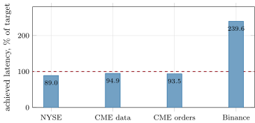
fig_plan.py, nw_plan.report().The missed target is the one the plan can fix cheaply. The configuration gives the crypto venue chapter 18’s three paths (an assumption about what it offers): its public endpoint through an edge network, and a private endpoint in the firm’s zone or in another zone. The plan tries each and ranks those that meet the target by cost.
def cheapest_fixes(plan, prices, bytes_per_month=0.0):
    """Each cloud venue missing its target: the offered paths that meet it, cheapest first."""
    fixes = []
    paths = pl.load_paths()
    for v in plan.venues:
        if v.access != "cloud" or latency_us(v, plan) <= v.target_us:
            continue
        for option in v.offers:
            alt = dataclasses.replace(v, path=option)
            x = latency_us(alt, plan)
            if x <= v.target_us:
                p = paths[option]
                extra = 12 * (p.usd_hour * 730 + p.usd_per_gb * bytes_per_month / 1e9)
                fixes.append({"venue": v.name, "option": option, "achieved_us": x,
                              "extra_annual": extra})
return sorted(fixes, key=lambda f: f["extra_annual"])A private endpoint in the instance’s zone brings the 99th-percentile round trip from to , for USD 122.64 a year of endpoint hours (at chapter 18’s price; its traffic charge adds to that with volume); one in another zone meets the target too, at , for the same fixed price plus cross-zone transfer. The fix is to align the endpoint with the instance’s zone identifier, chapter 16’s lesson.
29.3 The bill of materials
As of September 2026 — Prices in the plan, from the venues’ and the cloud’s published schedules
NYSE (schedule of 14 September 2026): dedicated cabinet 5 000 USD initial and 1 200 USD a kW a month at 4–8 kW; 10 Gb LCN and NMS network connection 15 000 USD initial and 24 000 a month (22 000 in NYSE’s October 2025 schedule, as Nasdaq’s filing cited it); cross connect 500 and 600 a month; wireless CME data 5 000 and 6 000 a month; CME data feed over the IP network 3 000 a month. Nasdaq’s comparable 10Gb Ultra connection: 18 500 USD a month from January 2026. AWS Tokyo (price list of 25 September 2026): c7i.4xlarge 0.8988 USD an hour.
| Item | Qty | Monthly (USD) | Annual (USD) | Source |
|---|---|---|---|---|
| NYSE dedicated cabinet (initial fee) | 1 | – | 1 667 | 29:F1 |
| NYSE cabinet power, 4–8 kW | 8 kW | 9 600 | 115 200 | 29:F1 |
| NYSE fibre cross connects | 4 | 2 400 | 29 467 | 29:F1 |
| NYSE 10 Gb LCN and NMS connection | 1 | 24 000 | 293 000 | 29:F1 |
| NYSE IP network 1 Gb (backup) | 1 | 2 500 | 30 833 | 15:F4 |
| Wavelength Mahwah–Aurora (CME orders) | 1 | 20 000 | 243 333 | assumed |
| NYSE wireless CME data | 1 | 6 000 | 73 667 | 29:F1 |
| CME data feed over the IP network | 1 | 3 000 | 36 000 | 29:F1 |
| AWS Tokyo c7i.4xlarge (730 h) | 2 | 1 312 | 15 747 | 29:F2 |
code/firm/connplan/data/cost_table.csv.Two checks run before the plan is trusted: every price row must name its ledger source, and none may be older than 60 days. On the day of writing, one row fails the first check, the Mahwah–Aurora wavelength, whose USD 20 000 a month is an assumption the firm must replace with a carrier’s quote; none fails the second. The table is also the plan’s export: export_cost_table writes it with its sources and dates for the firm’s budget owners (Book 16 reads it).
29.4 Contracts and service levels
The plan’s access to the equity venue is one 10 Gb connection, with a 1 Gb IP-network circuit as a backup. With each circuit failing once in 4 000 hours and repaired in four (assumptions), one connection alone is available 99.900% of the time; with the backup and a common-mode event (a shared duct or room) twice in ten years for eight hours, 99.982% (firm.slamodel, chapter 15). A second 10 Gb connection beside the backup would add USD 366 250 a year to the budget with the recovery share: the price of keeping full bandwidth through a failure. The fee schedule read for the plan mentions no service-level credits for these circuits; they belong in the contract.
29.5 The annual budget and its sensitivities
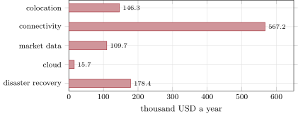
fig_plan.py, nw_plan.report().The plan costs USD 68 812 a month plus 39 500 in one-time fees: USD 1 017 289 a year with the fees amortised over three years and the recovery site at a quarter of the on-site spend. Connectivity is 56% of it, and one connection, the 10 Gb LCN and NMS link, is 29% alone. The sensitivities show where the budget moves: a second LCN connection adds USD 366 250 a year; four more kW of power 72 000; a wavelength priced 50% above the assumption 152 083; doubling the Tokyo instances only 15 747; dropping the backup circuit saves 38 542 and costs the availability above. The cloud leg, the one that missed its target, is the cheapest to fix and to grow.
Method 29.2 (Building and keeping a connectivity plan)
- Write the requirements as data: each venue, what each strategy needs from it, and the measure (percentile, one way or round trip).
- Compute each latency with the component that models its access; compare with the target and flag every miss.
- For each miss, try the offered alternatives and rank those that meet the target by cost.
- Price every line from a dated, sourced row; flag unsourced and stale rows and replace assumptions with quotes before signing.
- Add service levels and the recovery design; compute the budget and its sensitivities; export the cost table.
- Re-run the plan at every price change, venue move or new strategy: the plan is a program, not a document.
29.6 Tutorial: three venues, one budget
Goal. Run the whole plan from one configuration and change one requirement. End state: Tables 29.1 and 29.2 and Figure 29.2.
- Configuration.
nw_plan.VENUESandLINES(Listing 29.1) withfirm_connplan.load_prices. - Latency.
latency_table(Listing 29.2);cheapest_fixes(Listing 29.3). - Money.
bom,budget,check_prices,nw_plan.sensitivitiesandexport_cost_table.
What to change next. Tighten the equity target to and let the plan propose chapter 7’s hardware path; move the futures strategy to Aurora and compare the budgets.
29.7 Build: the connectivity plan
Purpose. The firm’s connectivity plan as a program: latency table, bill of materials, contracts, recovery line, budget, sensitivities, fixes, checks and the exported cost table. The book’s capstone.
Interface. firm_connplan: PriceRow, load_prices, Venue, Line, Plan, latency_us, latency_table, bom, budget, check_prices, cheapest_fixes, availability, export_cost_table; the exported table’s columns in its README.md.
Rules. Every price row names its ledger source and date, or is flagged; latencies come from the book’s components; targets and assumptions are stated in the configuration.
Acceptance tests. code/firm/connplan/tests/: price rows, a budget by hand, the checks and the fix on a small plan, a fibre route against its floor, and the exported table.
Stretch. Every access kind for every venue, with its alternatives priced; currency conversion with dated rates; the hardware path as an option for colocated venues.
Sources and further reading
- NYSE, Connectivity Fees and Charges (September 2026); Nasdaq, SR-NASDAQ-2025-089; AWS EC2 price list (Tokyo, September 2026).
- This book’s chapters 2 to 28 and their ledgers.
29.8 Exercises
Exercise 29.1 ★
What is a bill of materials, and what must each of its rows carry in this book’s plan?
Solution
Solution of Exercise 29.1.
The itemised list of everything the plan buys; each row carries the item, supplier, quantity, monthly and one-time price, the ledger row that publishes the price and the date it was read, or a flag that the price is an assumption.
Exercise 29.2 ★
What does an 8 kW dedicated cabinet cost a month in Mahwah on the September 2026 schedule?
Solution
Solution of Exercise 29.2.
USD a month, plus a 5 000 USD initial fee for the cabinet.
Exercise 29.3 ★
Why does the plan flag the Mahwah–Aurora wavelength?
Solution
Solution of Exercise 29.3.
Its price has no published source: the carrier does not publish it, so the plan carries an assumption, and the check that every price row names its source fails on it until the firm has a quote.
Exercise 29.4 ★★
How much of the annual budget is the 10 Gb LCN and NMS connection, and how much did its monthly price rise between NYSE’s October 2025 and September 2026 schedules?
Solution
Solution of Exercise 29.4.
USD 293 000 a year, 28.8% of the budget; its monthly price rose from 22 000 to 24 000 USD, by 9.1%.
Exercise 29.5 ★★
Why does a private endpoint in another zone meet the Tokyo target but still cost more than one in the instance’s zone?
Solution
Solution of Exercise 29.5.
Its round trip, at the 99th percentile, is under one millisecond, but traffic between the zones is charged each way per gigabyte on top of the endpoint’s hours, and the extra round trip leaves less margin.
Exercise 29.6 ★★
Which single change moves the budget most, and why is it not obviously worth it?
Solution
Solution of Exercise 29.6.
A second 10 Gb LCN connection, USD 366 250 a year; it buys full bandwidth through a connection failure, which the 1 Gb backup already covers at reduced bandwidth for 38 542 a year; its value depends on what trading at 1 Gb for a few hours a year costs.
Exercise 29.7 ★★★
Coding. With firm_connplan, what one-way latency does the CME order route reach with a route factor of 1.2 instead of 1.3?
Solution
Solution of Exercise 29.7.
, against at 1.3.
Exercise 29.8 ★★★
Find the flaw. “Our plan costs USD 1.02 million a year; we can sign today.”
Solution
Solution of Exercise 29.8.
One row is an assumption, not a price: the wavelength must be quoted, and at 50% above the assumption the budget rises by USD 152 083. The missed Tokyo target must be fixed, and the contracts’ service levels are not yet in the plan.
29.9 Problem: Three Venues, One Budget
Problem 29.1
Weekend problem — the capstone plan
The firm of the chapter must present its plan to its board. Use firm.connplan and the chapter’s configuration.
Part I — Latency.
- What does each venue achieve against its target?
- Which components computed each figure?
- Which of the figures are published and which modelled?
- What is missed, by how much, and why?
Part II — The fix.
- Which options meet the missed target, and at what latency?
- What does the cheapest cost a year?
- What must the firm check in its cloud account for the fix to work?
- Why is the fix so cheap compared with the rest of the plan?
Part III — Money.
- What are the monthly, one-time and annual costs?
- How is the annual cost split by category?
- Which row fails the checks, and what should the firm do?
- What do the sensitivities show?
Part IV — The verdict.
- State the named result: the annual all-in connectivity cost of entering the three venues, the latency achieved at each against its target, and the cheapest change that meets the one missed target.
- What does the backup circuit buy?
- What would moving the futures strategy to Aurora change?
- What should the board ask before approving?
- How often should the plan be re-run?
- What does Book 16 take from the plan?
- What part of the plan would you check first if a latency target were missed in production?
- In one sentence: what is a connectivity plan for?
Solution
Solution of Problem 29.1.
Part I.
- NYSE against 40; CME data against 4.2; CME orders against 8; Binance against 1.
- The cage and software path (
firm.cagenet,firm.wirepath); the published radio route;firm.fibrerouteon the geodesic;firm.privlink. - Published: the radio figure and the software stages’ measurements. Modelled: the cage, the cards, the fibre route factor, the cloud path’s edge time.
- The Tokyo round trip, 240% of target, because the public endpoint adds an edge network’s two milliseconds.
Part II.
- A private endpoint in the instance’s zone, ; one in another zone, .
- USD 122.64 a year of endpoint hours, plus its traffic charge.
- That the endpoint has an interface in the instance’s physical zone, by zone identifier, not name (chapter 16).
- It removes an edge network from the path rather than buying distance; the rest of the plan pays for distance and access.
Part III.
- USD 68 812 a month, 39 500 one-time, 1 017 289 a year.
- Connectivity 567 167, disaster recovery 178 375, colocation 146 333, market data 109 667, cloud 15 747.
- The wavelength’s price is unsourced: get carrier quotes and replace the assumption before signing.
- Bandwidth and redundancy on the equity connection and the wavelength’s price move the budget; the cloud barely does.
Part IV.
- Named result: USD 1.02 million a year all in (1 017 289), with NYSE at of a target, CME data at 3.986 of 4.2 and CME orders at 7.48 of , and Binance at against one; a private endpoint in the instance’s zone meets it at for USD 123 a year.
- Availability from 99.900% to 99.982% under the chapter’s assumptions, at reduced bandwidth during a failure.
- The order route shrinks to a cross-connect, the data route reverses (New Jersey prices to Chicago), and a second colocation footprint enters the budget.
- Which prices are quotes and which assumptions, which targets come from which strategies, and what each sensitivity is worth to the business.
- At every price change, venue move or new strategy, and at least before each contract renewal.
- The exported cost table, with each line’s source and date, to budget the firm’s technology tiers.
- The latency table’s component for that venue, then the path it assumed: route, zone, endpoint.
- To know, before signing, what the firm will get at each venue and what it will pay.
29.10 Interview questions
Interview question 29.1 ★ developer
What goes into a trading firm’s connectivity plan?
Solution
Solution of Interview question 29.1.
The venues and what each strategy needs from them; sites, routes, connections and services; their latency, service levels, recovery arrangements and cost, each price dated and sourced; the checks that keep it current.
What the interviewer is looking for: Requirements; latency; bill of materials; service levels; recovery; budget.
Interview question 29.2 ★★ developer
How would you estimate the latency from New Jersey to a futures exchange near Chicago before buying anything?
Solution
Solution of Interview question 29.2.
From the two sites’ coordinates: the geodesic, the fibre floor at the glass’s group index, a route factor from published routes, and equipment; compare with published radio figures for the same corridor.
What the interviewer is looking for: Geodesic; group index; route factor; published comparisons.
Interview question 29.3 ★★ developer, researcher
Your plan misses one latency target. How do you decide what to change?
Solution
Solution of Interview question 29.3.
List the alternatives that could meet it, compute each one’s latency with the same models, price each, and pick the cheapest that meets the target with margin; check whether the target itself is right.
What the interviewer is looking for: Alternatives; same models; cost ranking; margin.
Interview question 29.4 ★★ developer
How do you keep a plan’s prices trustworthy over time?
Solution
Solution of Interview question 29.4.
Every price is a dated row with its source; a check fails rows older than a limit and rows without a source; the plan is re-run when schedules change.
What the interviewer is looking for: Dated sources; staleness checks; automation.
Interview question 29.5 ★★ researcher
The board asks whether the second 10 Gb connection is worth USD 366 000 a year. How do you answer?
Solution
Solution of Interview question 29.5.
Estimate how often and how long the primary connection fails, what trading at the backup’s bandwidth loses in those hours, and compare that expected loss with USD 366 000 a year; include what the firm’s impact tolerance requires.
What the interviewer is looking for: Failure rates; loss while degraded; tolerance.
Interview question 29.6 ★★★ developer, researcher
Design the connectivity of a new firm trading U.S. equities, CME futures and a crypto venue in Tokyo, from requirements to budget.
Solution
Solution of Interview question 29.6.
Requirements per strategy; colocation at the equity venue; radio data and a fibre route for futures, or a second footprint near the futures exchange; instances in the crypto venue’s cloud zone with a private endpoint; service levels and a recovery site; a budget with sources, sensitivities and checks, re-run as prices change.
What the interviewer is looking for: All the book’s pieces; alternatives; sources; checks.