Markets III: Commodities, Energy and Crypto · Markets

1Physical Commodity Markets

A tanker finishes loading 700 000 barrels of North Sea crude on a Tuesday. The buyer and the seller signed their contract weeks ago, and neither of them yet knows the price. The contract says: the average of a published daily assessment of North Sea crude over five business days, two before the date on the loading document, that date, and two after, plus forty cents. Both parties will learn the price the following Monday evening, when the last of the five assessments is published. Until then the refinery that bought the oil holds a cargo whose cost moves every day, and it has to decide whether, and how, to fix it. This chapter describes the layer of the commodity world that such contracts make up, the physical market, and the tools by which traders turn its floating prices into the fixed prices a business can plan with.

1.1 Physical and paper

Commodity markets have two layers. One moves goods: ships, pipelines, tanks, silos and warehouses, with contracts that name a quality, a quantity, a place and a date. The other moves only money: futures, swaps and options whose settlement depends on a price. Books 1 and 2 of this series dealt almost entirely with the second kind of instrument; in commodities the first kind comes first, because it is where prices are made.

Definition 1.1 (Physical market, paper market)

The physical market of a commodity is the set of contracts for the delivery of a specified quantity and quality of the commodity at a specified place and time. Its paper market is the set of contracts on the commodity’s price that are normally settled in cash or closed out before delivery: futures, swaps and options.

The boundary is porous. A futures contract with physical delivery (One Quant Book 1, chapter 21) is paper for almost all of its life and physical at its end; an exchange for physical turns one into the other. The paper market’s own workhorse outside exchanges is the swap.

Definition 1.2 (Commodity swap)

A commodity swap exchanges, for each period of its life, a fixed price for the average of a published floating price over the period, both applied to an agreed volume, and is settled in cash for the difference.

Example 1.3 (A monthly crude swap)

An airline buys a swap on 100 000 barrels a month for the next quarter at a fixed $82.00\,\$/\mathrm{bbl}$ against the monthly average of a crude benchmark. If the benchmark averages $85.40\,\$/\mathrm{bbl}$ in the first month, the airline receives $3.40 \times 100\,000 = \$340\,000$ ; if it averages $79.10\,\$/\mathrm{bbl}$ in the second, it pays $\$290\,000$ . Whatever it pays for its fuel in the physical market, its net cost per barrel is fixed near $82, up to the difference between the fuel it burns and the benchmark it hedged, which is the subject of the last section.

1.2 Trading houses and the physical value chain

Between the producer that lifts a commodity and the consumer that burns, smelts or mills it stand firms that buy, store, blend, ship and resell.

Definition 1.4 (Commodity trading house)

A commodity trading house is a firm whose business is to buy physical commodities and resell them, earning the difference between their value in one place, time or form and their value in another, and hedging the flat price with paper.

A trading house transforms a commodity in three ways, each of which a price difference rewards: in space (a cargo bought at a loading port and sold at a discharge port), in time (oil stored when the forward price pays for the tank) and in form (grades blended into a specification a refinery wants). Pirrong’s study of the industry describes trading firms in exactly these terms, as performers of physical transformations, whose profits come from the spreads between locations, dates and qualities rather than from the level of prices. That is why a well-run trading house hedges almost all of its flat-price exposure: the level of oil prices is a risk it carries, not the one it is paid for.

As of September 2026 — How large the largest trader is

Vitol, among the largest energy traders, reported deliveries of 8 million barrels a day of crude oil and products in 2025 (7.2 million in 2024), on a turnover of USD 343 billion. World oil demand was about 104 million barrels a day; the International Energy Agency forecast in May 2026 that it would contract in 2026, to 104 million barrels a day, after shipments through the Strait of Hormuz were disrupted.

Remark 1.5 (Why the business is concentrated)

A physical trade ties up working capital for the whole voyage: a 700 000-barrel cargo at $80\,\$/\mathrm{bbl}$ is USD 56 million, paid on delivery and recovered weeks later. The firms that do this at scale are those with the bank credit lines to finance it (Chapter 13) and the flow to spread fixed costs over many cargoes.

1.3 Delivery terms and the physical contract

A physical contract must say where the goods change hands, who pays to move them, and who bears the risk of their loss on the way. International practice uses standard terms for this.

Definition 1.6 (Incoterms, free on board, cost insurance and freight)

Incoterms are the standard delivery terms published by the International Chamber of Commerce. Under free on board (FOB) the seller delivers the goods on board the vessel nominated by the buyer at the named port of shipment; risk passes there, and the buyer pays freight and insurance. Under cost insurance and freight (CIF) risk also passes on board at the port of shipment, but the seller contracts and pays for the carriage to the named destination port and for insurance against the buyer’s risk of loss.

Definition 1.7 (Bill of lading)

A bill of lading is the document the carrier issues on loading: a receipt for the goods, evidence of the contract of carriage, and a document of title whose holder may claim the cargo at destination. Its date, the B/L date, anchors most pricing formulas.

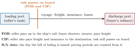
**Figure 1.1.** The two delivery terms of seaborne commodity trade. Under both, the buyer carries the risk of the voyage; under CIF the seller pays for it and prices that cost into the cargo. Schematic.

A CIF price is therefore approximately the FOB price plus freight and insurance: the two terms differ in who organises and pays for the voyage, not in who bears its risk. Beyond the Incoterm, a physical contract names the grade and its specification, the volume with an operational tolerance (a cargo is rarely exactly the size agreed), the loading or delivery date range, the inspection agent whose measurement of quantity and quality is binding, the payment terms (often by letter of credit, thirty days after the B/L date; Chapter 13) and the price formula.

1.4 Price-reporting agencies and assessment windows

Most physical cargoes do not trade on an exchange, so there is no exchange price to write into their formulas. The prices come from specialised publishers.

Definition 1.8 (Price-reporting agency, assessment window)

A price-reporting agency (PRA) is a publisher that assesses and publishes, every business day, the prices of physical commodities and related over-the-counter contracts from the bids, offers and trades it observes and from reports by market participants. An assessment window is a fixed daily period during which the agency collects bids, offers and trades that it then uses to set its assessment at the window’s closing time.

The two largest agencies in oil are Platts, part of S&P Global, and Argus. Their assessments are referenced by physical contracts and by the paper contracts that hedge them, and so work as benchmarks. In October 2012, at the request of the G20, the International Organization of Securities Commissions published principles for oil price-reporting agencies whose assessments are referenced by derivatives contracts: governance, the quality and integrity of the methodology, and the management of conflicts of interest.

As of September 2026 — The North Sea window

Platts assesses Dated Brent from its market-on-close process: bids, offers and trades reported during a thirty-minute window, 16:00 to 16:30 London time each business day, with the assessment reflecting the value of the most competitive grade at 16:30. Participants submit bids and offers for cargoes of specified size, loading dates and grade; the agency publishes them and the trades. A parallel window runs in Singapore for Middle-East crude.

1.5 Pricing formulas, netbacks and hedging a physical deal

Definition 1.9 (Pricing period, price differential)

The pricing period of a physical contract is the set of days whose benchmark assessments are averaged to set its price: for example the five business days around the B/L date (written 2-1-2), or all days of the delivery month. The price differential is the fixed premium or discount added to that average; it carries the value of the grade, location and timing relative to the benchmark, and is what the parties actually negotiate.

A trader who buys at one place and sells at another compares them through the value at a single point.

Definition 1.10 (Netback)

The netback of a sale is its delivered price less the costs of getting the commodity there (freight, insurance, losses in transit, duties and terminal fees), expressed per unit at the point of origin.

Example 1.11 (Choosing a destination by netback)

A cargo can be sold delivered in Rotterdam at $81.30\,\$/\mathrm{bbl}$ with $1.10\,\$/\mathrm{bbl}$ of freight, or in Singapore at $83.10\,\$/\mathrm{bbl}$ with $3.05\,\$/\mathrm{bbl}$ ; insurance costs $0.03\,\$/\mathrm{bbl}$ either way. The netbacks are $80.17\,\$/\mathrm{bbl}$ and $80.02\,\$/\mathrm{bbl}$ : Rotterdam, although Singapore pays more.

A physical formula leaves the parties exposed to the benchmark until the last pricing day. They hedge that exposure with paper on the same benchmark, or on a closely related one, and what the hedge cannot remove has a name.

Definition 1.12 (Basis risk)

Basis risk is the risk that the price of the position being hedged and the price of the hedging instrument move by different amounts: the risk that remains in a hedged position because the basis between them changes.

Method 1.13 (Hedging a cargo priced over a period)

When the price is fixed on $n$ pricing days, each day fixes $1/n$ of the volume. (i) On the day the exposure is created (the contract is signed and its price will float), take a futures position of the same size and opposite sign to the exposure that pricing will create: a buyer of floating-price oil who wants a fixed cost buys futures now. (ii) On each pricing day, close $1/n$ of the futures at that day’s settlement. (iii) The hedged price is then the futures price at inception plus the average basis over the pricing days plus the differential.

Proposition 1.14 (What a hedged cargo costs)

Let $F_d$ be the futures price and $b_d$ the physical-minus-futures basis on day $d$ , and let the pricing days be $d_1,\dots,d_n$ . A buyer hedged by Method 1.13 from day $0$ pays per barrel

\frac1n\sum_{i=1}^n (F_{d_i}+b_{d_i}) + D - \frac1n\sum_{i=1}^n (F_{d_i}-F_0) \;=\; F_0 + \frac1n\sum_{i=1}^n b_{d_i} + D ,

where $D$ is the differential. The flat price has gone; the average basis remains.

Proof. The formula price is the first average plus $D$ ; the futures bought at $F_0$ and sold in equal parts at $F_{d_i}$ gain the second average. Subtract. ∎

Figure 1.2 simulates the refinery of the hook: futures move by $1.80\,\$/\mathrm{bbl}$ a day and the basis by $0.12\,\$/\mathrm{bbl}$ a day, both as random walks. Unhedged, the cost of the cargo has a standard deviation of $8.13\,\$/\mathrm{bbl}$ , about USD 5.7 million on the cargo; hedged, of $0.54\,\$/\mathrm{bbl}$ , which is exactly the standard deviation of the average basis over the five pricing days.

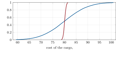
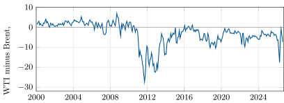
Distribution of the cost of a cargo priced 2-1-2 around a B/L date twenty business days away, with futures at 80\,\$/ bbl, a basis of -0.30\,\$/ bbl and a differential of +0.40\,\$/ bbl: 20 000 simulated paths. The hedge removes the flat price and leaves the basis. Illustrative volatilities; data: the chapter’s tutorial. — **Figure 1.2.** Distribution of the cost of a cargo priced 2-1-2 around a B/L date twenty business days away, with futures at $80\,\$/\mathrm{bbl}$ , a basis of $-0.30\,\$/\mathrm{bbl}$ and a differential of $+0.40\,\$/\mathrm{bbl}$ : 20 000 simulated paths. The hedge removes the flat price and leaves the basis. Illustrative volatilities; data: the chapter’s tutorial.

Basis risk is small when the hedge and the cargo reference the same benchmark and large when they do not. The largest physical benchmarks, the seaborne North Sea barrel and the inland US barrel (Chapter 2), move together most of the time and apart when logistics break (Figure 1.3). In 2011 inland US crude production outgrew the pipelines out of the storage hub at Cushing, Oklahoma, and the inland barrel fell to a monthly-average discount of about $27 in September 2011; in 2026 the seaborne barrel rose above it by as much as $17.66 in the April monthly average while shipments through the Strait of Hormuz were disrupted. A hedger who had sold one benchmark against a cargo priced on the other would have lost or gained those amounts on top of the flat price.

**Figure 1.3.** The inland US benchmark minus the seaborne North Sea benchmark, monthly averages of daily spot prices, January 2000 to August 2026. The pipeline bottleneck of 2011 and the Gulf disruption of 2026 are the two deepest discounts. Data: FRED series DCOILWTICO and DCOILBRENTEU (US Energy Information Administration).

1.6 Tutorial: pricing and hedging a cargo

Goal. Price a cargo from its formula, hedge it by Method 1.13, and measure what the hedge leaves. End state: Figure 1.2 and the standard deviations $8.13\,$ and $0.54\,\$/\mathrm{bbl}$ .

The legs and the hedge. A leg is bought or sold, priced over a set of days; each pricing day fixes an equal share and the hedge trades that share.

@dataclass(frozen=True)
class Leg:
    """One side of a physical deal: +1 bought, -1 sold; priced over `days`."""
    side: int
    volume: float
    days: tuple[int, ...]
    differential: float


def fixed_fraction(leg: Leg, day: int) -> float:
    """Share of the leg's volume whose price is fixed at the close of `day`."""
    return sum(1 for d in leg.days if d <= day) / len(leg.days)


def exposure(legs: list[Leg], day: int) -> float:
    """Flat-price exposure in barrels at the close of `day`: the priced (fixed) part of every leg.
    A floating leg carries no flat-price risk: its price will move with the market."""
    return sum(leg.side * leg.volume * fixed_fraction(leg, day) for leg in legs)


def hedge_trades(legs: list[Leg], lot: int = LOT) -> dict[int, int]:
    """Futures lots to trade at each pricing day's close so that the hedge offsets the exposure:
    as a bought leg prices in, sell; as a sold leg prices in, buy (positive = buy)."""
    trades: dict[int, int] = {}
    for leg in legs:
        per_day = leg.volume / len(leg.days) / lot
        if abs(per_day - round(per_day)) > 1e-9:
            raise ValueError("volume per pricing day is not a whole number of lots")
        for d in leg.days:
            trades[d] = trades.get(d, 0) - leg.side * round(per_day)
    return {d: q for d, q in sorted(trades.items()) if q}

Listing 1.1. Legs, exposure and the futures trades that offset it. code/firm/physdeal/firm_physdeal.py

Simulate. Futures and basis as random walks; cost unhedged and hedged, and the theoretical hedged standard deviation from the covariance of a random walk.

def simulate_cargo(n_paths: int = 20_000, seed: int = 1) -> dict[str, np.ndarray]:
    """Cost per barrel of the refiner's cargo, unhedged and hedged, on simulated paths.
    Physical assessment = futures + basis; both are random walks from today (day 0)."""
    rng = np.random.default_rng(seed)
    days = pricing_days(BL_DAY, 2, 2)
    horizon = max(days) + 1
    f = F0 + np.cumsum(rng.normal(0.0, SIGMA_F, (n_paths, horizon)), axis=1)
    b = B0 + np.cumsum(rng.normal(0.0, SIGMA_B, (n_paths, horizon)), axis=1)
    physical = (f + b)[:, days].mean(axis=1) + DIFF          # the formula price
    hedge_gain = (f[:, days] - F0).mean(axis=1)              # bought 700 lots today, sold 140 a day
    return {"unhedged": physical, "hedged": physical - hedge_gain}


def hedged_sd_theory() -> float:
    """Standard deviation of the hedged cost: that of the average basis over the pricing days."""
    days = np.array(pricing_days(BL_DAY, 2, 2)) + 1          # steps taken by day d (day 0 is one step)
    cov = SIGMA_B ** 2 * np.minimum.outer(days, days)
    return float(np.sqrt(cov.sum()) / len(days))

Listing 1.2. The refinery’s cargo on 20 000 paths. code/markets-3/01-physical-commodity-markets/python/m3_physical.py

Run m3_physical.simulate_cargo(), hedged_sd_theory() and fig_physical.py.

What to change next. Hedge on the bill-of-lading date only, instead of over the pricing period, and measure the residual; replace the basis random walk by a mean-reverting one and see how much of the hedged risk remains.

1.7 Build: the physical deal model

Purpose. Every physical trade of the miniature firm enters its books through this model: what the price will be, which days still float, what freight and insurance the firm pays, and which futures to trade each day to keep the book flat.

Interface. pricing_days(event_day, before, after); formula_price(assessments, days, differential); Leg(side, volume, days, differential); exposure(legs, day); hedge_trades(legs); cost_split(incoterm, freight, insurance); netback; locked_margin.

Rules. Days are business-day indices; a missing assessment is an error, never an interpolation; each pricing day fixes an equal share; futures lots are whole (1 000 barrels) or the schedule is rejected; FOB and CIF only.

Acceptance tests. code/firm/physdeal/tests/: a 2-1-2 period; the exposure of a back-to-back cargo is zero before and after both pricing periods and the full volume between them; hedge plus exposure is zero on every day; netback and the Incoterm split.

Stretch. Post the futures trades to the position keeper of One Quant Book 1, chapter 7; price-date calendars with holidays; volume tolerance at the buyer’s option.

Sources and further reading

International Chamber of Commerce, Incoterms 2020; ICC Academy, “Place of delivery and risk transfer in international trade contracts”.
IOSCO, Principles for Oil Price Reporting Agencies, FR06/12, 5 October 2012 (Internet Archive copy), and the implementation report of 2013.
S&P Global Platts, Dated Brent methodology and the market-on-close process.
C. Pirrong, The Economics of Commodity Trading Firms, 2014.
Vitol, 2025 volumes and review; IEA, Oil Market Report, May and August 2026.
US Energy Information Administration, Today in Energy, “Spread narrows between Brent and WTI crude oil benchmark prices”, 2013; FRED series DCOILWTICO and DCOILBRENTEU.

1.8 Exercises

Exercise 1.1 ★

A cargo is priced at the average of five assessments plus $0.35\,\$/\mathrm{bbl}$ . The assessments are 81.20, 80.70, 79.90, 80.40 and 81.05. What is the price?

Solution

Solution of Exercise 1.1.

The five assessments sum to 403.25, an average of 80.65; plus 0.35, the price is $81.00\,\$/\mathrm{bbl}$ .

Exercise 1.2 ★

A seller offers a cargo at $78.40\,\$/\mathrm{bbl}$ FOB. Freight to the buyer’s port is $1.35\,\$/\mathrm{bbl}$ and insurance $0.04\,\$/\mathrm{bbl}$ . What CIF price is equivalent, and who bears the risk of the voyage under each term?

Solution

Solution of Exercise 1.2.

$78.40 + 1.35 + 0.04 = 79.79\,\$/\mathrm{bbl}$ CIF. Under both terms the risk passes to the buyer when the oil is on board at the loading port: the buyer bears the voyage risk either way; under CIF the seller pays for the freight and the insurance that covers the buyer.

Exercise 1.3 ★

A cargo sells delivered at $84.10\,\$/\mathrm{bbl}$ ; freight is $2.20\,\$/\mathrm{bbl}$ , insurance $0.05\,\$/\mathrm{bbl}$ , and 0.2% of the volume is lost in transit. Give the netback per barrel loaded.

Solution

Solution of Exercise 1.3.

$84.10 \times 0.998 - 2.20 - 0.05 = 81.68\,\$/\mathrm{bbl}$ .

Exercise 1.4 ★★

A refinery buys 700 000 barrels priced 2-1-2 around the B/L date. How many 1 000-barrel futures does it buy today, and how many does it sell on each pricing day? What changes if one of the five days is a holiday on which no assessment is published and the contract drops it?

Solution

Solution of Exercise 1.4.

It buys 700 futures today and sells 140 on each pricing day. If a day is dropped the price is the average of four assessments: it sells 175 on each of the four days.

Exercise 1.5 ★★

In the simulation of Figure 1.2 the hedged standard deviation is $0.54\,\$/\mathrm{bbl}$ . What would it be if the daily volatility of the basis doubled, and why does the futures volatility not enter?

Solution

Solution of Exercise 1.5.

$1.08\,\$/\mathrm{bbl}$ : the hedged cost is $F_0$ plus the average basis plus the differential (Proposition 1.14), whose standard deviation is proportional to the basis volatility. The futures moves are bought and sold back on the same days as the physical prices in, so they cancel exactly.

Exercise 1.6 ★★

Using Example 1.11, by how much would Singapore’s delivered price have to rise for the trader to switch destinations?

Solution

Solution of Exercise 1.6.

The netbacks are 80.17 (Rotterdam) and 80.02 (Singapore): Singapore’s delivered price must rise by more than $0.15\,\$/\mathrm{bbl}$ , to above $83.25\,\$/\mathrm{bbl}$ .

Exercise 1.7 ★★★

Coding. With load_differential, find the month of the deepest WTI discount to Brent since 2000 and its size, and count the months since January 2011 in which WTI averaged above Brent.

Solution

Solution of Exercise 1.7.

September 2011, $-27.31\,\$/\mathrm{bbl}$ ; WTI averaged above Brent in 4 of the months from January 2011 to August 2026 (115 of all 320 months since 2000, almost all before 2011).

Exercise 1.8 ★★★

Find the flaw. “Our cargo prices around the B/L date, so we hedge it by buying 700 futures on the B/L date and selling them once the price is known.” Correct it.

Solution

Solution of Exercise 1.8.

The cargo’s cost starts to float when the contract is signed, not on the B/L date, and it fixes one fifth a day over the five pricing days, two of which come before the B/L date. Buy the 700 futures when the exposure is created and sell 140 on each pricing day at that day’s settlement; selling them all “once the price is known” leaves the last days’ futures moves unmatched by any physical move.

1.9 Problem: The Cargo That Priced Late

Problem 1.1

Weekend problem — a back-to-back cargo with two pricing periods

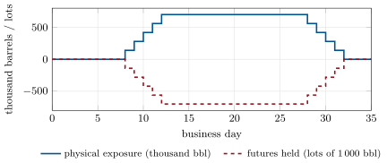
A trading house buys 700 000 barrels FOB, priced 2-1-2 around the B/L date (day 10) at Dated plus $0.20\,\$/\mathrm{bbl}$ , and sells the same cargo CIF Rotterdam, priced 2-1-2 around the discharge date (day 30) at Dated plus $1.10\,\$/\mathrm{bbl}$ . It pays freight of $0.65\,\$/\mathrm{bbl}$ and insurance of $0.03\,\$/\mathrm{bbl}$ . Dated moves by about $1.80\,\$/\mathrm{bbl}$ a business day.

Part I — The exposure.

What is the trader’s flat-price exposure before day 8?
How does it change on days 8 to 12?
What is it between days 13 and 27, and for how many days is it at its maximum?
How does it change on days 28 to 32?
Sketch the exposure against time.

Part II — The hedge.

What futures does the trader trade on each of days 8 to 12?
And on days 28 to 32?
What is the net futures position on day 20?
Why is no futures position needed before day 8?
Which instrument would you use if the futures did not settle on Dated?

Part III — The money.

Give the margin per barrel locked in by the hedge.
Give it for the cargo, in dollars.
Estimate the standard deviation of the unhedged P&L.
What risks remain after the hedge?
How does a delay of the discharge by five days change the exposure and the hedge?

Part IV — Judgement.

Why might the trader choose a CIF sale rather than FOB?
What does the trader’s credit line have to finance?
Why do trading houses call this business “spread” trading?
State the named result: the locked margin of the cargo against its unhedged risk.
In one sentence: what does a physical trader earn?

Solution

Solution of Problem 1.1.

1. Zero: both prices float with Dated. 2. It rises by 140 000 barrels a day as the purchase prices in, to 700 000 long on day 12. 3. 700 000 barrels long, from day 12 to day 27: 16 days. 4. It falls by 140 000 a day to zero on day 32. 5. A trapezoid (Figure 1.4). 6. Sell 140 futures a day. 7. Buy back 140 a day. 8. Short 700. 9. A floating purchase against a floating sale has no flat-price exposure. 10. A swap on the Dated average of each pricing period (a Dated-to-futures swap, Chapter 2), or futures plus the residual basis. 11. $1.10 - 0.20 - 0.65 - 0.03 = 0.22\,\$/\mathrm{bbl}$ . 12. $154 000. 13. Twenty business days between the pricing periods: $1.80\sqrt{20} \times 700\,000 \approx$ USD 5.63 million. 14. The basis between Dated and the futures at each pricing day, volume tolerance, demurrage and delays, counterparty credit, and operational losses. 15. The sale prices on days 33–37: the exposure lasts 21 days at its maximum and the buy-backs move five days later; the hedge must be kept open, and the futures may need rolling. 16. To capture the freight and the destination premium, and to control the voyage. 17. The purchase price, paid about thirty days after loading, until the sale proceeds arrive, plus the margin on the futures. 18. Its P&L is the differential between two prices, not the price level. 19. Named result: $154 000 locked per cargo ( $0.22\,\$/\mathrm{bbl}$ ) against an unhedged standard deviation of about USD 5.63 million. 20. The spread between a commodity’s value in two places, times or forms, less the cost of moving it, not the price level.

**Figure 1.4.** The weekend problem’s back-to-back cargo: the flat-price exposure builds as the purchase prices in (days 8–12) and unwinds as the sale prices in (days 28–32); the futures position mirrors it. Data: the chapter’s code.

1.10 Interview questions

Interview question 1.1 ★ trader

What is the difference between FOB and CIF, and which carries the voyage risk?

Solution

Solution of Interview question 1.1.

FOB: the seller loads onto the buyer’s ship and the buyer pays freight and insurance. CIF: the seller pays freight and insurance to the destination. In both the risk passes on board at the loading port, so the buyer bears the voyage risk.

What the interviewer is looking for: the distinction between who pays and who bears the risk.

Interview question 1.2 ★ trader, researcher

Why are most physical cargoes priced as an average over several days rather than at a single price?

Solution

Solution of Interview question 1.2.

An average is harder to move by one trade or one bad day, spreads the pricing over the time the cargo is actually loaded or delivered, and lets both sides hedge day by day in liquid paper.

What the interviewer is looking for: manipulation resistance, matching the operational window, hedgeability.

Interview question 1.3 ★★ trader, risk

You bought a cargo priced on the average of next month. When do you hedge, and how much each day?

Solution

Solution of Interview question 1.3.

At the trade date, hedge the whole volume, because the exposure exists as soon as the price will float; then close $1/n$ of the hedge on each of the $n$ pricing days (the month’s business days). A monthly average swap does this in one instrument.

What the interviewer is looking for: exposure created at signing, unwound by pricing days, the swap as the natural hedge.

Interview question 1.4 ★★ researcher

A price-reporting agency’s assessment and an exchange’s settlement price are both “the price”. How do they differ as data?

Solution

Solution of Interview question 1.4.

The settlement is computed by rule from exchange trades and is reproducible; the assessment is a judgement by an editorial team on bids, offers and trades in a window, sometimes with few trades, and can be revised. Its methodology, window and timestamp matter, and its history is licensed data.

What the interviewer is looking for: reproducibility, methodology risk, licensing.

Interview question 1.5 ★★ risk

A trading house says it hedges all its flat-price risk. Where can it still lose money?

Solution

Solution of Interview question 1.5.

On basis between the benchmark hedged and the cargo’s formula, on timing mismatches (delays, tolerances), on counterparty default, on operational losses and demurrage, and on the financing of margin calls on its hedges while the physical gain is unrealised.

What the interviewer is looking for: basis, operations, credit and liquidity rather than flat price.

Interview question 1.6 ★★★ developer, trader

Design the service that tells a physical desk, every evening, its exposure by benchmark and pricing day and the futures it should hold.

Solution

Solution of Interview question 1.6.

Deal capture with each leg’s formula, benchmark and pricing days; a calendar of business days per benchmark; a nightly job that computes the fixed fraction of each leg, aggregates exposure by benchmark and day, compares it with futures and swaps held, and outputs the trades to flatten; alerts on missing assessments and on legs whose dates move.

What the interviewer is looking for: the leg-and-pricing-day data model, per-benchmark aggregation, reconciliation with hedges.

Terms defined in this chapter

See all 2333 terms in the glossary