Markets III: Commodities, Energy and Crypto · Markets

5Power Markets I: Design

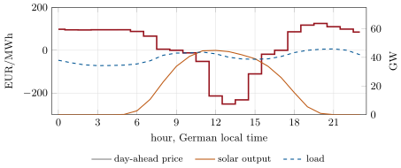
On Sunday 11 May 2025, between 13:00 and 14:00, German solar panels produced 44 gigawatts while the whole country consumed 40. The day-ahead auction had cleared that hour the day before at minus 250 euros a megawatt-hour: producers paid to deliver electricity, and consumers were paid to take it. Five months earlier, at 17:00 on a windless 12 December 2024, the same auction had cleared at 936 euros. Electricity is the one commodity that must be produced at the moment it is consumed, and power markets are designed around that fact. This chapter describes the design: the market time unit, the day-ahead auction and how its algorithm clears, the merit order that sets the price, zones and nodes, and the markets for capacity and reserves that energy prices alone do not pay for.

5.1 Electricity as a commodity

Electricity can hardly be stored at scale, and supply and demand on a grid must match at every instant or its frequency drifts from its nominal 50 or 60 hertz. Markets therefore trade energy for delivery over short, fixed intervals, and the grid operator balances whatever remains in real time.

Definition 5.1 (Market time unit)

The market time unit (MTU) is the delivery interval of a power market’s products: an energy product is a constant power delivered over one MTU, so a quantity of energy in MWh per MTU.

A power market is a sequence of markets for the same MTU: forwards and futures for months and years ahead, the day-ahead auction, continuous intraday trading (Chapter 6), and the operator’s balancing in real time. The day-ahead auction is the anchor: most volume in Europe is priced there, and most forwards settle against its prices.

5.2 The day-ahead auction and its clearing algorithm

Definition 5.2 (Day-ahead market)

The day-ahead market is a daily sealed-bid call auction, held the day before delivery, that sets for each MTU of the next day one uniform-price clearing (One Quant Book 2, chapter 4) per bidding zone from the buy and sell orders submitted before its gate closure.

For each MTU, buyers submit a stepwise demand curve (how much they will buy at each price) and sellers a stepwise supply curve. The algorithm chooses the accepted orders that maximise welfare, the value of the accepted bids minus the cost of the accepted offers, subject to the network constraints between zones, and sets in each zone the price at which supply and demand cross. Every accepted order is paid or pays that price; nobody pays their bid.

Proposition 5.3 (The clearing price supports the allocation)

At the clearing price $p$ of a single zone with stepwise curves, every accepted bid has a limit $\ge p$ and every accepted offer a limit $\le p$ ; no rejected bid has a limit above $p$ and no rejected offer a limit below $p$ . The accepted volume maximises welfare.

Proof. Serving bids in decreasing and offers in increasing price order and stopping when the next bid is worth less than the next offer adds each unit of positive surplus and no unit of negative surplus: that is the welfare maximum. The marginal order, partly filled, sets $p$ , which by construction lies between the limits of the accepted and the rejected orders on each side. ∎

Real auctions add orders that span several MTUs.

Definition 5.4 (Block order)

A block order is an order to buy or sell a quantity in each of several MTUs, all or nothing, with a limit on the average price over those MTUs.

Blocks let a thermal plant, with its start-up cost and minimum run time, bid its true economics. They make clearing a combinatorial problem: a block may be rejected although the prices it would have received average above its limit (a paradoxically rejected block), but never accepted when they average below it. Europe’s day-ahead auctions are cleared by one algorithm across the whole continent.

Definition 5.5 (Market coupling)

Market coupling is the joint clearing of the day-ahead auctions of several zones by one algorithm, which allocates the cross-border transmission capacity implicitly: electricity flows from the low-price zone to the high-price zone until prices converge or the capacity is used up.

As of September 2026 — European day-ahead coupling

The Single Day-Ahead Coupling runs one auction at 12:00 CET for delivery the next day, cleared by the EUPHEMIA algorithm across all participating bidding zones. It moved from 60-minute to 15-minute market time units on trading day 30 September 2025, for delivery from 1 October 2025. The harmonised clearing-price limits were $-500\,\mathrm{EUR}/\mathrm{MWh}$ and $+4000\,\mathrm{EUR}/\mathrm{MWh}$ ; ACER’s Decision 02/2026 revised the methodology, and the minimum was lowered to $-600\,\mathrm{EUR}/\mathrm{MWh}$ from trading day 28 May 2026.

5.3 The merit order, spark and dark spreads

Definition 5.6 (Merit order)

The merit order is the ranking of generating capacity by short-run marginal cost, lowest first; with offers at marginal cost, the supply curve of the auction is the merit order and the price is the marginal cost of the last plant needed.

A thermal plant’s marginal cost is its fuel cost per MWh of electricity plus the cost of the allowances for its emissions (Chapter 7): $(P_{\mathrm{fuel}} + e\,P_{\mathrm{CO_2}})/\eta$ , with $\eta$ its efficiency and $e$ the emissions per MWh of fuel. Wind and solar have almost none.

Definition 5.7 (Spark spread, dark spread)

The spark spread of a gas-fired plant of efficiency $\eta$ is the power price minus the price of the gas it burns per MWh of electricity, $P_{\mathrm{power}} - P_{\mathrm{gas}}/\eta$ ; the dark spread is the same for a coal-fired plant.

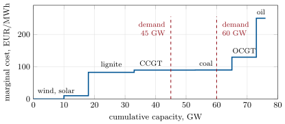
An illustrative merit order with 10 GW of wind and solar: gas at 35\, EUR/ MWh of fuel, coal at 12\,, lignite at 5\,, carbon at 70\, EUR/ t. At 45 GW of demand a combined-cycle gas plant sets the price (89.35\, EUR/ MWh); at 60 GW a coal plant does (89.68\,). Data: the chapter’s tutorial. — **Figure 5.1.** An illustrative merit order with 10 GW of wind and solar: gas at $35\,\mathrm{EUR}/\mathrm{MWh}$ of fuel, coal at $12\,$ , lignite at $5\,$ , carbon at $70\,\mathrm{EUR}/\mathrm{t}$ . At 45 GW of demand a combined-cycle gas plant sets the price ( $89.35\,\mathrm{EUR}/\mathrm{MWh}$ ); at 60 GW a coal plant does ( $89.68\,$ ). Data: the chapter’s tutorial.

With the fuels of Figure 5.1 and power at $100\,\mathrm{EUR}/\mathrm{MWh}$ , a 55%-efficient gas plant earns a spark spread of $36.36\,\mathrm{EUR}/\mathrm{MWh}$ and a 40%-efficient coal plant a dark spread of $70.00\,$ before carbon: after carbon the coal plant is dearer (Chapter 7). Adding renewables shifts the whole stack to the right and lowers the price in every hour in which they produce: with 30 GW of wind and solar and 60 GW of demand the price falls from $89.68\,$ to $89.35\,\mathrm{EUR}/\mathrm{MWh}$ ; with 55 GW, to $10\,\mathrm{EUR}/\mathrm{MWh}$ .

5.4 Zonal and nodal pricing

A network has limits, and a price must say where it applies.

Definition 5.8 (Bidding zone)

A bidding zone is the largest geographic area within which market participants can trade energy without allocating transmission capacity; the day-ahead market sets one price per zone and MTU.

Europe prices by zones, mostly national; the United States’ organised markets price by nodes.

Definition 5.9 (Locational marginal price, congestion rent)

The locational marginal price (LMP) at a node of a network is the cost of serving one more MWh there at least cost, subject to the network’s limits: in US markets the sum of a system energy price, a congestion component and a loss component. The congestion rent on a constrained line is the price difference between its ends times the flow on it; it accrues to whoever holds the line’s capacity rights (in coupled markets, the grid operators).

Proposition 5.10 (Two zones, one line)

Two zones cleared jointly through a line of capacity $C$ have equal prices if the flow that equalises them is at most $C$ . Otherwise the flow is $C$ from the cheap zone to the dear one, each zone clears alone with that flow as a price-taking export or import, and the congestion rent is $(p_B - p_A)\,C$ .

Proof. Joint clearing maximises total welfare. If the unconstrained optimum’s flow fits the line it is feasible and optimal, with one price. If not, welfare is concave in the flow, so the constrained optimum puts the flow at its bound; each zone then clears with the fixed flow, and the prices differ by the shadow price of the line. ∎

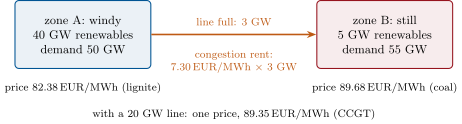
Two coupled zones with the merit order of . A 3 GW line is congested and prices split; the grid operators collect about EUR 21\,900 for the hour. With a 20 GW line prices converge. Data: the chapter’s tutorial. — **Figure 5.2.** Two coupled zones with the merit order of Figure 5.1. A 3 GW line is congested and prices split; the grid operators collect about EUR $21\,900$ for the hour. With a 20 GW line prices converge. Data: the chapter’s tutorial.

Zonal pricing hides congestion inside a zone, which the operator must then relieve by redispatch, paying some plants to produce less and others more; nodal pricing reveals it in the price but gives thousands of prices instead of one, and exposes every generator to the local congestion of its node. The next chapter shows how traders hedge that exposure.

5.5 Capacity markets, ancillary services and negative prices

An energy-only market pays generators only for the MWh they sell. A plant that runs a few hours a year must earn its fixed costs in those hours, at scarcity prices, which regulators often cap.

Definition 5.11 (Capacity market, ancillary service)

A capacity market pays resources for being available to produce (or to reduce consumption) in future periods of system stress, through auctions held years ahead, with penalties if they fail to deliver. An ancillary service is a service other than energy that the grid operator buys to keep the system secure: frequency reserves that respond in seconds to minutes, voltage support, and the ability to restart the grid after a blackout.

The price cap and the capacity market are two answers to the same problem. The Texas market, energy-only, set its price at its cap of $9000\,\$/\mathrm{MWh}$ for days in February 2021 during a winter storm; the regulator’s order was challenged in court and upheld by the Supreme Court of Texas in 2024. The market monitor found that holding prices at the cap for 32 hours after load shedding ended, until the morning of 19 February, added USD 16 billion to the market’s costs.

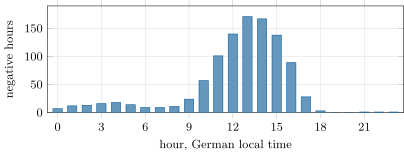
At the other end, prices go below zero when supply that will not or cannot stop exceeds demand plus export capacity. Three kinds of producers keep producing at negative prices: plants whose shutdown and restart cost more than the loss of running through a few hours; producers paid a subsidy per MWh produced, who produce as long as the price plus the subsidy is positive; and plants that must run for other reasons (heat for a town, system security). On 11 May 2025 German solar output exceeded the country’s load in five hours (Figure 5.3). In the German data, 457 hours had a negative average price in 2024 and 573 in 2025 (hourly averages, as the Bundesnetzagentur also counts them; from October 2025 the auction clears quarter-hours), almost all in the middle of the day (Figure 5.4).

Germany on Sunday 11 May 2025, hourly: the day-ahead price (left axis) fell to -250.32\, EUR/ MWh at 13:00 while solar output (right axis) exceeded load from 11:00 to 16:00. Data: Bundesnetzagentur | SMARD.de, CC BY 4.0. — **Figure 5.3.** Germany on Sunday 11 May 2025, hourly: the day-ahead price (left axis) fell to $-250.32\,\mathrm{EUR}/\mathrm{MWh}$ at 13:00 while solar output (right axis) exceeded load from 11:00 to 16:00. Data: Bundesnetzagentur | SMARD.de, CC BY 4.0.

**Figure 5.4.** German day-ahead hours with a negative price, 2024 and 2025 together (1 030 hours), by local hour of delivery: the solar hours dominate. Data: Bundesnetzagentur | SMARD.de, CC BY 4.0.

5.6 Tutorial: clearing an hour and coupling two zones

Goal. Clear one MTU from stepwise orders, then couple two zones through a line. End state: the prices of Figures 5.1 and 5.2 and the negative hours of Figure 5.4.

One zone. Merit-order matching and the marginal order’s price.

def clear(orders: list[Order]) -> Result:
    """Uniform-price clearing of one MTU. Bids are served in decreasing price order, offers in
    increasing price order, while the next bid is worth at least the next offer. The price is that
    of the marginal order: the one left partly unfilled (an offer if both are exhausted together).
    `fills` gives the accepted quantity of each order, in input order."""
    idx_b = sorted((k for k, o in enumerate(orders) if o.side == BUY), key=lambda k: -orders[k].price)
    idx_o = sorted((k for k, o in enumerate(orders) if o.side == SELL), key=lambda k: orders[k].price)
    fills = [0.0] * len(orders)
    i = j = 0
    volume = welfare = 0.0
    price = None
    while i < len(idx_b) and j < len(idx_o):
        b, o = orders[idx_b[i]], orders[idx_o[j]]
        if b.price < o.price:
            break
        rb, ro = b.qty - fills[idx_b[i]], o.qty - fills[idx_o[j]]
        q = min(rb, ro)
        fills[idx_b[i]] += q
        fills[idx_o[j]] += q
        volume += q
        welfare += q * (b.price - o.price)
        price = b.price if rb > ro else o.price
        if rb <= ro + 1e-12:
            i += 1
        if ro <= rb + 1e-12:
            j += 1
    if price is None:
        raise ValueError("curves do not cross")
    return Result(price, volume, welfare, tuple(fills))

Listing 5.1. Uniform-price clearing of one market time unit. code/firm/dayahead/firm_dayahead.py

Two zones. Proposition 5.10.

def couple(zone_a: list[Order], zone_b: list[Order], capacity: float) -> dict[str, float]:
    """Two zones and one interconnector of `capacity` MWh in each direction. Clear both zones as one
    market; if the implied flow fits the line, both zones get the common price. Otherwise the line
    is full: each zone clears alone with the flow as a price-taking export or import, prices split,
    and the congestion rent is the price difference times the flow."""
    joint = clear(zone_a + zone_b)
    fa = joint.fills[:len(zone_a)]
    flow = sum(f for f, o in zip(fa, zone_a, strict=True) if o.side == SELL) - \
        sum(f for f, o in zip(fa, zone_a, strict=True) if o.side == BUY)
    if abs(flow) <= capacity + 1e-9:
        return {"flow": flow, "price_a": joint.price, "price_b": joint.price, "rent": 0.0}
    f = capacity if flow > 0 else -capacity
    pa = clear(zone_a + [Order(BUY, 1e6, f)] if f > 0 else zone_a + [Order(SELL, -1e6, -f)]).price
    pb = clear(zone_b + [Order(SELL, -1e6, f)] if f > 0 else zone_b + [Order(BUY, 1e6, -f)]).price
    return {"flow": f, "price_a": pa, "price_b": pb, "rent": (pb - pa) * f}

Listing 5.2. Two zones coupled through one line. code/firm/dayahead/firm_dayahead.py

Run m3_power.hour(60, 10), two_zones(3), negative_stats() and fig_power.py.

What to change next. Raise the carbon price until coal and gas swap places in the merit order; add a block offer for a lignite plant over the solar hours and see whether it is accepted.

5.7 Build: the day-ahead clearing engine

Purpose. The miniature firm bids plants and batteries into day-ahead auctions and must predict the prices its own bids help set: it needs a clearing engine it can run on its own forecasts of everyone else’s curves.

Interface. Order(side, price, qty); clear(orders) -> Result(price, volume, welfare, fills); couple(zone_a, zone_b, capacity); Block(name, price, qty, mtus); clear_with_blocks(hourly, blocks); marginal_cost; spark_spread; dark_spread.

Rules. Uniform price per zone and MTU; the partly filled marginal order sets the price; curves that do not cross are an error; a block is all-or-nothing and never paradoxically accepted; enumeration is limited to small block sets (the real algorithm uses branch and bound).

Acceptance tests. code/firm/dayahead/tests/: the marginal offer sets the price; a negative price; congestion splits prices and earns the rent; convergence with a large line; a dear block rejected.

Stretch. More than two zones on a meshed network with flow-based constraints; 15-minute MTUs with hourly blocks; the price-limit rules of the dated box.

Sources and further reading

EPEX SPOT and the Market Coupling Steering Committee, notices on the 15-minute MTU in SDAC (2025); ENTSO-E, Single Day-ahead Coupling.
ACER Decision 02/2026 on the harmonised maximum and minimum clearing price for SDAC; SDAC communication note of 7 May 2026.
PJM, Formation of Locational Marginal Pricing and its System Energy, Congestion and Loss Components.
Supreme Court of Texas, decision of June 2024 on the PUCT’s February 2021 pricing orders (via Reed Smith client note).
Potomac Economics (ERCOT’s independent market monitor), recommendation to the PUCT, Project No. 51812, 4 March 2021 (Internet Archive copy).
Bundesnetzagentur | SMARD.de: day-ahead prices DE-LU, generation and load, 2024–2025; Bundesnetzagentur, press release on the electricity market in 2025.

5.8 Exercises

Exercise 5.1 ★

Offers: 300 MWh at $0\,$ , 200 at $40\,$ , 200 at $90\,$ , 100 at $150\,\mathrm{EUR}/\mathrm{MWh}$ . Demand bids 450 MWh at the price cap. Give the price and the accepted volume of each offer.

Solution

Solution of Exercise 5.1.

$40\,\mathrm{EUR}/\mathrm{MWh}$ : the 300 MWh at zero and 150 of the 200 MWh at 40 are accepted, the offer at 40 being marginal; the offers at 90 and 150 are rejected.

Exercise 5.2 ★

A gas plant of efficiency 50% burns gas at $30\,\mathrm{EUR}/\mathrm{MWh}$ and emits 0.202 t per MWh of gas; carbon costs $70\,\mathrm{EUR}/\mathrm{t}$ . What is its marginal cost?

Solution

Solution of Exercise 5.2.

$(30 + 0.202 \times 70)/0.5 = 88.28\,\mathrm{EUR}/\mathrm{MWh}$ .

Exercise 5.3 ★

Why does every accepted seller receive the clearing price rather than its own offer? What would sellers do under pay-as-bid?

Solution

Solution of Exercise 5.3.

In a uniform-price auction all accepted energy is worth the same at the margin, and sellers can bid their marginal cost: any accepted offer earns the clearing price. Under pay-as-bid each seller would bid what it expects the marginal price to be, not its cost, so the offers would no longer reveal the merit order; the auction format itself is studied in One Quant Book 4, chapter 29.

Exercise 5.4 ★★

In Figure 5.2, what are the flow, the prices and the congestion rent if the line’s capacity is 3 GW? What minimum capacity makes the prices converge?

Solution

Solution of Exercise 5.4.

Flow 3 GW from A to B, prices $82.38\,$ and $89.68\,\mathrm{EUR}/\mathrm{MWh}$ , rent $7.30 \times 3\,000 \approx$ EUR 21 900 for the hour (EUR 21 890 with the unrounded price gap, $7.297\,\mathrm{EUR}/\mathrm{MWh}$ ). Zone A has 63 GW of capacity cheaper than $89.35\,$ against 50 GW of demand: with more than 13 GW of line, its gas plants can export too and the prices converge at $89.35\,\mathrm{EUR}/\mathrm{MWh}$ .

Exercise 5.5 ★★

A solar farm receives a premium of $60\,\mathrm{EUR}/\mathrm{MWh}$ on top of the market price for every MWh it produces. Below what price does it stop? In which hours of 11 May 2025 would it have stopped?

Solution

Solution of Exercise 5.5.

It produces while the price plus the premium is positive: it stops below $-60\,\mathrm{EUR}/\mathrm{MWh}$ , that is in the four hours from 12:00 to 16:00 on 11 May 2025 (prices from $-212.82$ to $-110.06$ ).

Exercise 5.6 ★★

Explain why nodal prices differ inside a zone that has one zonal price, and who pays for the difference in a zonal system.

Solution

Solution of Exercise 5.6.

Inside a zone the network still has limits; the nodal price, which includes congestion, differs across them, but the zonal market ignores this and clears at one price. The operator then redispatches, paying plants on one side of the bottleneck to reduce and on the other to increase output, and the cost is recovered through network charges from all consumers.

Exercise 5.7 ★★★

Coding. With negative_stats, give the number of negative hours in 2024 and in 2025, the local hour with the most, and the lowest price and its hour.

Solution

Solution of Exercise 5.7.

457 in 2024 and 573 in 2025; the most at 13:00 local time (171 over the two years); the lowest price $-250.32\,\mathrm{EUR}/\mathrm{MWh}$ at 13:00 on 11 May 2025.

Exercise 5.8 ★★★

Find the flaw. “Negative prices prove the market is broken: nobody should ever pay to produce.”

Solution

Solution of Exercise 5.8.

A negative price says that at that hour one more MWh has negative value: supply that cannot or will not stop exceeds demand. It pays flexible consumers to consume and flexible producers to stop, which is the market working; producers that keep producing do so because stopping costs more (restarts) or because they are paid per MWh produced (subsidies).

5.9 Problem: The Day with Too Much Sun

Problem 5.1

Weekend problem — 11 May 2025 from a lignite unit

A lignite unit of the merit order of Figure 5.1 (marginal cost $82.38\,\mathrm{EUR}/\mathrm{MWh}$ ) can run no lower than 400 MW. On 11 May 2025 the German day-ahead prices were negative from 09:00 to 18:00 local time.

Part I — The day.

In how many hours was the price negative, and what was their average?
What was the lowest price, and when?
In which hours did solar output exceed load?
Where did the surplus go?
Why did the auction not clear at zero?

Part II — The unit.

What does the unit lose, relative to not producing, in one hour at minimum load at the lowest price?
What does it lose over the nine negative hours at minimum load?
Why does it compare this loss with its restart cost?
State the rule for staying on.
What bid would express that rule in the auction?

Part III — The subsidised producers.

A solar farm with a premium of $60\,\mathrm{EUR}/\mathrm{MWh}$ produces in which negative hours?
What price does a large block of such farms put on the auction?
How have subsidy rules been changed to limit this?
Why does battery storage raise midday prices?
Which producers profit from negative prices?

Part IV — Judgement.

What would an interconnector twice as large have done to the German price that day?
Why are negative prices concentrated in spring?
What is the value of a flexible consumer on such a day?
State the named result: the restart cost below which the unit should switch off.
In one sentence: what does a negative power price signal?

Solution

Solution of Problem 5.1.

1. Nine hours, average $-98.54\,\mathrm{EUR}/\mathrm{MWh}$ . 2. $-250.32\,$ , 13:00 to 14:00. 3. From 11:00 to 16:00 (five hours). 4. Exports to neighbouring zones up to the lines’ capacity, storage (pumped hydro, batteries), and curtailment of producers that stop at negative prices. 5. Supply bid below zero, from producers who lose more by stopping or are paid per MWh produced, exceeded demand at zero. 6. $400 \times (82.38 + 250.32) =$ EUR 133 080. 7. $400 \times \sum_h (82.38 - p_h) =$ EUR 651 308 over the nine hours. 8. Switching off avoids that loss but costs a restart (fuel to warm up, wear, and the risk of not being ready for the evening peak). 9. Stay on if the restart cost exceeds the loss of running at minimum load through the negative hours. 10. A block offer over the day at minimum load with a limit that includes the restart cost, or offers at negative prices for the minimum load. 11. Every negative hour whose price is above $-60$ : 9:00, 10:00, 11:00, 16:00 and 17:00. 12. About $-60\,\mathrm{EUR}/\mathrm{MWh}$ : their offers sit at minus their premium. 13. By paying no premium when prices are negative: in Germany, for new solar plants since February 2025, in every negative quarter-hour, so such producers bid at zero or stop. 14. It buys (charges) in the cheapest hours, adding demand there, and sells in the evening. 15. Flexible consumers, storage, and producers that can stop and buy back their forward sales cheaply. 16. More export would have raised the German price and lowered the neighbours’, until the line filled or the prices met. 17. Strong sun, mild temperatures and holidays give high solar output against low demand. 18. It is paid to consume: its value is the negative price times the consumption it can shift. 19. Named result: the unit should switch off if restarting costs less than EUR 651 308. 20. That the system has more inflexible supply than demand at that hour, and pays anyone who can absorb it or stop.

5.10 Interview questions

Interview question 5.1 ★ trader

How is the day-ahead power price in a European zone set?

Solution

Solution of Interview question 5.1.

By a daily sealed-bid auction at noon for each MTU of the next day: bids and offers form stepwise curves, one algorithm clears all coupled zones together, maximising welfare subject to cross-border capacities, and each zone gets a uniform price where its curves cross.

What the interviewer is looking for: uniform price, welfare maximisation, market coupling.

Interview question 5.2 ★ trader, researcher

What is the merit order, and how does adding wind change prices?

Solution

Solution of Interview question 5.2.

The supply stack sorted by marginal cost. Wind has near-zero marginal cost, so it shifts the stack right and the demand line meets it lower: prices fall in windy hours, and more so where the stack is steep.

What the interviewer is looking for: shift of the stack, cannibalisation of windy hours.

Interview question 5.3 ★★ researcher

You want to forecast tomorrow’s day-ahead price for each hour. What inputs matter, and which is most important in spring?

Solution

Solution of Interview question 5.3.

Load, wind and solar forecasts (residual load), fuel and carbon prices, plant availability, interconnector capacities and neighbours’ residual load, calendar effects. In spring, solar and wind forecasts dominate midday prices.

What the interviewer is looking for: residual load as the key feature; weather.

Interview question 5.4 ★★ trader, risk

Why can a power price be negative, and how deep can it go?

Solution

Solution of Interview question 5.4.

When inflexible or subsidised supply exceeds demand plus exports: producers pay to avoid restart costs or to keep subsidies. The auction’s harmonised minimum bounds it (in Europe $-500\,$ , then $-600\,\mathrm{EUR}/\mathrm{MWh}$ from May 2026).

What the interviewer is looking for: mechanisms, and knowledge of the floor.

Interview question 5.5 ★★ researcher

Compare zonal and nodal pricing from the point of view of a wind farm owner.

Solution

Solution of Interview question 5.5.

Under zonal pricing it receives the zone’s price whatever local congestion does, but may be curtailed by redispatch; under nodal pricing it receives its node’s price, which falls when local lines are congested, so it bears the congestion risk and needs transmission rights to hedge.

What the interviewer is looking for: who bears congestion risk, and the hedge.

Interview question 5.6 ★★★ developer, researcher

Design a day-ahead clearing simulator for ten zones and 96 MTUs with block orders. How do you keep it fast enough to run thousands of scenarios?

Solution

Solution of Interview question 5.6.

A welfare-maximisation problem with network constraints (a linear or quadratic programme per scenario) plus a combinatorial layer for blocks (branch and bound, or a heuristic with paradox checks). Speed: warm-start from the previous scenario, decompose by day, vectorise the per-MTU curves, and cache block decisions that do not change.

What the interviewer is looking for: LP plus combinatorics, and practical acceleration.

Terms defined in this chapter

See all 2333 terms in the glossary