Markets III: Commodities, Energy and Crypto · Markets

20Automated Market Makers

A pool holds ether and dollars and quotes no prices. Anyone may send it one token and take out the other, in any amount, provided that after the trade the product of its two balances is no smaller than before. That single rule, written in a few dozen lines of a smart contract, makes a market: the price is the ratio of the balances, a buyer pushes it up by taking ether out, and arbitrageurs keep it in line with the price on centralised exchanges by trading whenever the two differ. Those who deposit the balances earn the fees and bear a cost that is less obvious than the fees and, for most pools, larger. This chapter explains the automated market maker: the constant-product rule and its concentrated variant, the invariant used for stablecoins, what liquidity providers earn and lose, measured the way the recent literature measures it, and the routers and auctions that sit between traders and pools.

20.1 Constant-product market makers

Definition 20.1 (Decentralised exchange, automated market maker, liquidity pool)

A decentralised exchange is a trading venue implemented as smart contracts on a blockchain, on which users trade from their own wallets and every trade settles on chain. An automated market maker is a decentralised exchange whose prices are set by a formula applied to the balances of a liquidity pool: a contract holding reserves of two or more tokens, deposited by liquidity providers who receive a claim on them and on the fees.

Definition 20.2 (Constant-product market maker)

A constant-product market maker is an automated market maker whose pool of reserves $x$ and $y$ accepts a trade only if $xy$ does not decrease, with a fee $\gamma_{\mathrm{fee}}$ taken on the input and left in the pool.

Proposition 20.3 (Swap output and marginal price)

A trader who sends $\Delta x$ to a constant-product pool with reserves $(x, y)$ and fee $\gamma_{\mathrm{fee}}$ receives

\Delta y = \frac{y\,(1 - \gamma_{\mathrm{fee}})\,\Delta x}{x + (1 - \gamma_{\mathrm{fee}})\,\Delta x}.

The pool’s marginal price of the first token is $y/x$ ; the average price of the trade is $\Delta y / \Delta x$ , below $y/x$ by the fee and by a price impact that grows with $\Delta x / x$ . Without the fee, the product is exactly preserved; with it, the product grows.

Proof. Only $(1 - \gamma_{\mathrm{fee}})\Delta x$ counts towards the invariant: $(x + (1 - \gamma_{\mathrm{fee}})\Delta x)(y - \Delta y) = xy$ gives $\Delta y$ . The fee part of $\Delta x$ is added to the reserves on top, so $(x + \Delta x)(y - \Delta y) > xy$ . The marginal price is $-dy/dx$ along $xy = k$ , equal to $y/x$ . ∎

A pool of 1 000 ether and 3 million dollars quotes ether at 3 000 dollars. Selling it 10 ether with a 0.30% fee returns 29 614.74 dollars, an average of 2 961.47: 128 basis points below 3 000, of which 30 are the fee and about 98 the impact. The pool has no bid and no offer; its “spread” is twice the fee plus the impact of the size, and its depth is set by its reserves. Its price moves only when someone trades with it. When ether moves on centralised exchanges, the pool’s price is stale until an arbitrageur trades it back into line, and the arbitrageur’s profit comes out of the pool.

As of September 2026 — Fee tiers and versions of the largest AMM

Uniswap v2 charges a fee of 30 basis points on trades, paid to liquidity providers. Uniswap v3 (whitepaper dated March 2021, deployed to Ethereum mainnet on 5 May 2021) introduced concentrated liquidity and fee tiers, initially 0.05%, 0.30% and 1% with tick spacings of 10, 60 and 200 ticks, where a tick is a price step of a factor 1.0001. Uniswap v4 became operational on 31 January 2025, adding hooks, modular plugins that let developers add custom logic for pools, swaps, fees and positions. By CoinGecko’s count, spot volume on decentralised exchanges rose from 6.0% of centralised exchanges’ spot volume in January 2021 to a peak of 37.4% in June 2025, and stood near 21% in November 2025.

20.2 Concentrated liquidity

Definition 20.4 (Concentrated liquidity)

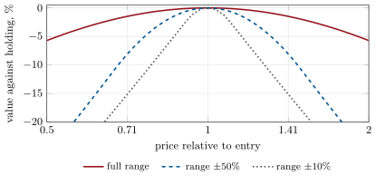
Concentrated liquidity is liquidity provided to an automated market maker over a chosen price range only: the position behaves as a constant-product pool with a larger virtual reserve while the price is inside the range, and holds only one of the two tokens when the price is outside it.

In Uniswap v3 a position is a liquidity amount $L$ over a range $[P_a, P_b)$ . Inside the range, with square-root price $\sqrt{P}$ , it holds $L(1/\sqrt{P} - 1/\sqrt{P_b})$ of the first token and $L(\sqrt{P} - \sqrt{P_a})$ of the second; below $P_a$ it holds only the first token, above $P_b$ only the second. Prices are stored as square roots in binary fixed point, and ranges end on ticks. A narrow range needs far fewer tokens than a full-range position for the same $L$ , so the same capital provides more depth near the current price: a range of $\pm10\%$ is about 21 times as capital-efficient as the full range. It also sells its tokens faster as the price moves through the range, and it earns nothing once the price has left it.

Impermanent loss: value of a liquidity position against simply holding the tokens deposited, after the price moves by a factor, for a full-range constant-product position and for concentrated positions over ±50\% and ±10\% around the entry price. The narrower the range, the faster the loss accrues; outside the range the position holds only the token that has lost value against the other. Data: the chapter’s tutorial. — **Figure 20.1.** Impermanent loss: value of a liquidity position against simply holding the tokens deposited, after the price moves by a factor, for a full-range constant-product position and for concentrated positions over $\pm50\%$ and $\pm10\%$ around the entry price. The narrower the range, the faster the loss accrues; outside the range the position holds only the token that has lost value against the other. Data: the chapter’s tutorial.

20.3 Stableswap

For two stablecoins that should trade at one for one, the constant product wastes liquidity: most of it sits at prices far from one that should never trade.

Definition 20.5 (Stableswap)

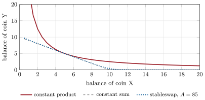
A stableswap market maker is an automated market maker whose invariant behaves like a constant sum (no price impact) near balanced reserves and like a constant product far from balance, blended by an amplification coefficient $A$ : for $n$ coins with balances $x_i$ and invariant $D$ ,

A n^n \sum_i x_i + D = A D n^n + \frac{D^{n+1}}{n^n \prod_i x_i}.

The invariant is solved numerically, for $D$ when liquidity is added and for one balance when a trade is made, by integer Newton iterations. With $A$ large the pool trades near one for one over a wide range of balances; if one coin depegs, arbitrageurs sell it into the pool until the pool holds mostly that coin, and the price then moves as in a constant-product pool. The liquidity providers of a stablecoin pool are therefore sellers of a put on the weaker coin’s peg.

**Figure 20.2.** Three invariants through the balanced point (5, 5), after the stableswap paper’s own comparison: the price is the slope. The stableswap curve follows the constant sum over a wide range of balances and bends into a constant-product shape only when one coin runs short. Curve’s integer solver. Data: the chapter’s tutorial.

20.4 Impermanent loss and loss-versus-rebalancing

Definition 20.6 (Impermanent loss)

The impermanent loss of a liquidity position is the difference between its value and the value of the tokens originally deposited, had they simply been held, after a price change; it is “impermanent” only in that it vanishes if the price returns to its starting level.

Proposition 20.7 (Impermanent loss of a constant-product position)

If the price of the first token moves by a factor $r$ , a full-range constant-product position is worth $2\sqrt{r}/(1 + r)$ times what holding its initial tokens would be worth. A halving or a doubling of the price costs 5.7%.

Proof. With liquidity $L = \sqrt{xy}$ , the pool holds $L/\sqrt{P}$ and $L\sqrt{P}$ and is worth $2L\sqrt{P}$ in the second token. Starting at $P_0$ and moving to $rP_0$ , the pool is worth $2L\sqrt{rP_0}$ , and the held tokens $L/\sqrt{P_0} \cdot rP_0 + L\sqrt{P_0} = L\sqrt{P_0}(1 + r)$ . The ratio is $2\sqrt{r}/(1 + r)$ . ∎

Impermanent loss mixes two things: exposure to the price, which a hedger could remove, and a genuine cost. Milionis, Moallemi, Roughgarden and Zhang separate them. Compare the pool with a portfolio that holds, at every instant, the same quantity of the risky token as the pool, bought and sold at market prices as the pool’s holding changes: the rebalancing portfolio has the same market risk as the pool.

Definition 20.8 (Loss-versus-rebalancing)

Loss-versus-rebalancing (LVR) is the difference between the value of a rebalancing portfolio that tracks an automated market maker’s holdings by trading at market prices and the value of the pool itself; it is the amount the pool loses to arbitrageurs by trading at its own stale prices rather than at the market’s.

Proposition 20.9 (LVR of a constant-product pool)

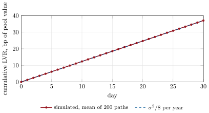
If the market price follows a geometric Brownian motion (One Quant Book 4) with volatility $\sigma$ and arbitrageurs keep a fee-free constant-product pool at the market price, LVR accrues at the instantaneous rate $\sigma^2/8$ per unit of time, as a fraction of the pool’s value. At a daily volatility of 5%, about 3.1 basis points of pool value a day.

Proof. The paper’s general result is an instantaneous LVR of $\tfrac12\sigma^2P^2\,|x^{*\prime}(P)|$ , with $x^*(P)$ the pool’s holding of the risky token. For the constant product, $x^* = L/\sqrt{P}$ , $|x^{*\prime}| = \tfrac12 L P^{-3/2}$ , and the rate is $\tfrac14 L\sigma^2\sqrt{P}$ ; divided by the pool value $2L\sqrt{P}$ it is $\sigma^2/8$ . ∎

LVR is the liquidity providers’ adverse selection (One Quant Book 1, chapter 19): every arbitrage trade is with someone who knows the price has moved. It depends on volatility, not on volume. Fees are what the pool earns from everyone else. The tutorial checks the closed form by simulation: on 200 lognormal paths with 60% annual volatility, rebalanced every 15 minutes for 30 days, the measured LVR averages 37.1 basis points of pool value against 37.0 from the formula.

Loss-versus-rebalancing of a fee-free constant-product pool: the rebalancing portfolio minus the pool, averaged over 200 simulated paths at 60% annual volatility with arbitrage every 15 minutes, against the closed form of ; the two lines coincide. Data: the chapter’s tutorial. — **Figure 20.3.** Loss-versus-rebalancing of a fee-free constant-product pool: the rebalancing portfolio minus the pool, averaged over 200 simulated paths at 60% annual volatility with arbitrage every 15 minutes, against the closed form of Proposition 20.9; the two lines coincide. Data: the chapter’s tutorial.

Proposition 20.10 (When fees pay for LVR)

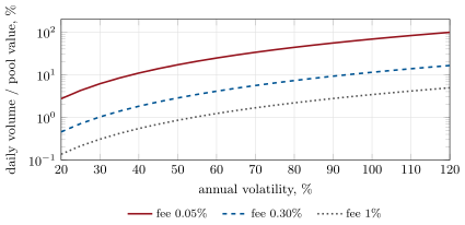
If noise traders turn over a volume $V$ a day through a constant-product pool of value $W$ with fee $\gamma_{\mathrm{fee}}$ , the pool’s fee income covers its LVR when $V/W \ge \sigma_d^2/(8\gamma_{\mathrm{fee}})$ , where $\sigma_d$ is the daily volatility.

Proof. Fee income is $\gamma_{\mathrm{fee}}V$ a day and LVR $\tfrac18\sigma_d^2 W$ a day; compare them. ∎

At 60% annual volatility, a 0.30% pool must turn over 4.1% of its value every day in non-arbitrage volume just to cover LVR; a 0.05% pool, 24.7%. Figure 20.4 shows the requirement across volatilities. Concentrating liquidity raises fee income and LVR in the same proportion while the price is in range, so it does not change the ratio; it changes how much capital is at stake and how often the position must be moved.

The daily turnover by noise traders at which a constant-product pool’s fees equal its loss-versus-rebalancing (), for three fee tiers. Data: the chapter’s tutorial. — **Figure 20.4.** The daily turnover by noise traders at which a constant-product pool’s fees equal its loss-versus-rebalancing (Proposition 20.10), for three fee tiers. Data: the chapter’s tutorial.

20.5 Just-in-time liquidity, aggregators and intent-based routing

Concentrated liquidity allows a strategy that only a blockchain’s ordering makes possible.

Definition 20.11 (Just-in-time liquidity)

Just-in-time liquidity is concentrated liquidity added in a narrow range immediately before a large pending swap, in the same block, and removed immediately after it, so as to earn most of the swap’s fee while bearing almost none of the pool’s arbitrage losses.

A just-in-time provider sees the swap in the mempool (Chapter 14), and needs its own transactions ordered before and after it: it is a form of the ordering games of Chapter 22. It takes fees from the pool’s passive providers and gives the trader a better price.

Definition 20.12 (DEX aggregator, intent-based routing)

A DEX aggregator splits a swap across several pools and venues to minimise the trader’s total cost of price impact, fees and gas. Intent-based routing lets the trader sign a message stating what he will give and the least he will accept, and lets competing third parties (fillers, solvers) find the execution and submit it on chain.

As of September 2026 — Two intent-based protocols

UniswapX’s documentation describes signed orders that specify a swap’s outputs, filled by competing fillers who use their own liquidity or route through other sources; on some chains the order is a Dutch auction whose price decays from a maximum to a minimum over time, and the swapper pays no gas and nothing for failed swaps. CoW Protocol’s documentation describes signed intents grouped into batches, with third-party solvers competing to find the best execution for each batch, first by matching opposite intents within it (a “coincidence of wants”) and otherwise by routing through AMMs, aggregators and private market makers.

For a trading firm the consequences are two. As a taker, it can often do better through an aggregator or an intent than against any single pool, and must compare them net of gas. As a liquidity provider or filler, it competes with specialised firms for the order flow of intents, a business much closer to the request-for-quote market making of One Quant Book 2 than to passive pool provision.

20.6 Tutorial: swaps, impermanent loss and LVR

Goal. Implement integer constant-product and stableswap swaps, compare a liquidity position with holding, and measure loss-versus-rebalancing by simulation against $\sigma^2/8$ . End state: the four figures of this chapter and the numbers of the weekend problem.

The swap. Proposition 20.3 in on-chain integer arithmetic.

def cp_amount_out(amount_in: int, reserve_in: int, reserve_out: int, fee_bps: int = 30) -> int:
    """Output of a constant-product swap; the fee stays in the pool (floor division, as on chain)."""
    a = amount_in * (10_000 - fee_bps)
    return a * reserve_out // (reserve_in * 10_000 + a)


def cp_amount_in(amount_out: int, reserve_in: int, reserve_out: int, fee_bps: int = 30) -> int:
    """Input needed for an exact output (rounded up by one unit, as on chain)."""
    return reserve_in * amount_out * 10_000 // ((reserve_out - amount_out) * (10_000 - fee_bps)) + 1

Listing 20.1. The constant-product swap, exact input and exact output. code/firm/amm/firm_amm.py

LVR. Hold the pool’s risky position in a rebalancing portfolio and compare.

def lvr_path(sigma: float, days: int, steps_per_day: int, seed: int) -> tuple[list[float], float]:
    """Arbitrageurs move a fee-free constant-product pool to the market price at every step of a driftless
    lognormal path. Returns the cumulative LVR (rebalancing portfolio minus pool, as a fraction of the
    initial pool value) at the end of each day, and the closed form sigma^2/8 per year integrated."""
    rng = random.Random(seed)
    dt = 1 / (365 * steps_per_day)
    p, liq = 1.0, 1.0
    pool0 = 2 * liq * math.sqrt(p)
    rebal, out, theory = pool0, [], 0.0
    for _ in range(days):
        for _ in range(steps_per_day):
            x, v_before, p_before = liq / math.sqrt(p), 2 * liq * math.sqrt(p), p
            p *= math.exp(-0.5 * sigma * sigma * dt + sigma * math.sqrt(dt) * rng.gauss(0, 1))
            rebal += x * (p - p_before)                     # hold the pool's risky position, rebalance
            theory += sigma * sigma / 8 * dt * v_before
        out.append((rebal - 2 * liq * math.sqrt(p)) / pool0)
    return out, theory / pool0

Listing 20.2. Loss-versus-rebalancing along one simulated path. code/markets-3/20-automated-market-makers/python/m3_amm.py

Run lvr_mean(), breakeven_turnover(0.6, 0.003) and fig_amm.py.

What to change next. Give the pool a fee and let arbitrageurs trade only when the mispricing exceeds it; measure how LVR falls with the block time; simulate a concentrated position that is re-centred when the price leaves its range and count what re-centring costs.

20.7 Build: the AMM library

Purpose. The miniature firm must price swaps exactly as the contracts will execute them (to the last unit), value its liquidity positions, and simulate sandwiches and lending liquidations against pools (Chapters 22 and 23).

Interface. cp_amount_out, cp_amount_in; tick_at_price, sqrt_price_x96, amounts_for_liquidity, next_sqrt_price_from_amount0; ss_get_d, ss_get_y, ss_amount_out. The Rust crate firm_amm implements the constant-product and stableswap functions in u128.

Rules. Integers only in token base units; floor division where the contracts floor, rounding up where they round up; square-root prices in Q64.96; Newton iterations capped and raising if they do not converge.

Acceptance tests. code/firm/amm/tests/ and the Rust crate’s tests: the swap formula and the growth of the invariant with fees; ticks and position amounts at the range edges; the price move after adding a token; stableswap balance and low slippage against the constant product; one swap with the same output in Python and Rust.

Stretch. Exact tick math in 256-bit integers; multi-range swaps crossing ticks; fees and LVR for a re-centred concentrated position.

Sources and further reading

H. Adams, N. Zinsmeister and D. Robinson, Uniswap v2 Core, 2020; H. Adams et al., Uniswap v3 Core, March 2021; Uniswap Labs, “Uniswap v4 is here”, 2025.
M. Egorov, StableSwap — efficient mechanism for Stablecoin liquidity, 2019.
J. Milionis, C. C. Moallemi, T. Roughgarden and A. L. Zhang, “Automated Market Making and Loss-Versus-Rebalancing”, arXiv:2208.06046, version of May 2026.
UniswapX and CoW Protocol documentation, September 2026; Uniswap Labs, “Uniswap v3 Mainnet launch”, 5 May 2021; CoinGecko Research, “DEX to CEX Volume Ratios”, updated 17 April 2026.

20.8 Exercises

Exercise 20.1 ★

A pool holds 1 000 ether and 3 000 000 dollars with a 0.30% fee. What does selling it 10 ether return? What is the average price?

Solution

Solution of Exercise 20.1.

$3\,000\,000 \times 9.97/(1\,000 + 9.97) = 29\,614.74$ dollars, an average of 2 961.47.

Exercise 20.2 ★

What is the impermanent loss of a full-range position when the price rises by a factor of 4?

Solution

Solution of Exercise 20.2.

$2\sqrt4/(1 + 4) - 1 = -20\%$ .

Exercise 20.3 ★

Why does a stableswap pool’s liquidity provider effectively sell a put on each coin’s peg?

Solution

Solution of Exercise 20.3.

If one coin depegs, arbitrageurs sell it into the pool at close to one for one until the pool holds mostly that coin: the providers end up owning the fallen coin, bought near par, as the writer of a put struck near par would.

Exercise 20.4 ★★

Annual volatility is 80%. What is the LVR of a constant-product pool per day and per year, as a fraction of pool value?

Solution

Solution of Exercise 20.4.

$0.8^2/8 = 8\%$ of pool value a year, about 2.19 basis points a day.

Exercise 20.5 ★★

A pool of USD 50 million with a 0.05% fee trades USD 20 million a day of non-arbitrage volume at 50% annual volatility. Do fees cover LVR?

Solution

Solution of Exercise 20.5.

LVR: $50\text{ million} \times 0.25/365/8 = \$4\,281$ a day; fees: $20\text{ million} \times 0.05\% = \$10\,000$ . Yes: turnover of 40% against a requirement of 17.1%.

Exercise 20.6 ★★

Explain why impermanent loss and LVR have the same expectation under the risk-neutral measure but are not the same thing.

Solution

Solution of Exercise 20.6.

Under the risk-neutral measure the rebalancing portfolio’s expected gain is zero, so the expected pool-versus-hold difference equals the expected LVR. But impermanent loss also contains the market-risk difference between the pool and holding the initial tokens, which a hedge removes; LVR is what remains after hedging, and it accrues path by path whatever the price does.

Exercise 20.7 ★★★

Coding. With lvr_path, rebalance every hour instead of every 15 minutes. Does the measured LVR change? What if you rebalance once a day?

Solution

Solution of Exercise 20.7.

About 37.0, 37.0 and 37.7 basis points over 30 days with 400 paths, every 15 minutes, hourly and daily. Without fees the expected LVR does not depend on how often the arbitrage happens: the pool’s value $2L\sqrt{P}$ loses $1 - e^{-\sigma^2t/8}$ in expectation whatever the steps (36.9 basis points here). With fees, less frequent arbitrage lets larger gaps build before trading, and the frequency then matters.

Exercise 20.8 ★★★

Find the flaw. “Our pool earned 12% a year in fees, so providing liquidity returned 12%.”

Solution

Solution of Exercise 20.8.

Fees are only the income side. The return also includes the loss to arbitrageurs (LVR) and the market exposure of the tokens held; net of LVR and hedged, the return can be negative although fees were 12%.

20.9 Problem: Should You Provide Liquidity?

Problem 20.1

Weekend problem — fees against loss-versus-rebalancing

A firm considers providing USD 10 million of liquidity to an ether–dollar constant-product pool with a 0.30% fee. Ether’s annual volatility is 60%. The pool, USD 200 million in all, trades USD 6 million a day of non-arbitrage volume.

Part I — The costs.

What is the pool’s daily LVR as a fraction of its value, and in dollars for the firm’s share?
What are the firm’s daily fees?
What daily turnover would make the fees cover LVR?
What is the firm’s expected annual result, ignoring market risk?
What happens to the answer if volatility doubles?

Part II — The alternatives.

Would the 0.05% tier with the same volume be better or worse?
Would a concentrated $\pm10\%$ range change the ratio of fees to LVR?
What does the firm do with its market risk, and what does it cost?
What volume would it need at 1% fee?
How does just-in-time liquidity change the passive provider’s fees?

Part III — Measurement.

How would you measure the pool’s non-arbitrage volume?
How would you measure LVR from the pool’s history?
Why does the block time matter for LVR?
What does impermanent loss over a month tell you about LVR?
What would you monitor once the position is live?

Part IV — Judgement.

Who wins in this pool, and who loses?
Is passive liquidity provision a market-making business?
Why do pools with high volume and low volatility attract liquidity?
State the named result: the daily turnover at which fees cover LVR at 60% volatility and a 0.30% fee, and whether this pool clears it.
In one sentence: what does a liquidity provider sell?

Solution

Solution of Problem 20.1.

1. $0.6^2/365/8 = 1.23$ basis points a day; USD 1 233 a day on USD 10 million. 2. $6\text{ million} \times 0.30\% \times 10/200 = \$900$ . 3. 4.11% of pool value a day, USD 8.2 million for this pool. 4. $(900 - 1\,233) \times 365 \approx -\$121\,500$ . 5. LVR quadruples: about $-\$1.47$ million a year. 6. Worse at the same volume: fees fall to $150 a day; a lower fee must attract several times the volume to pay. 7. No: while the price is in range, fees and LVR both scale with the concentration. 8. Hedges the ether exposure (short perpetuals or futures sized to the pool’s ether holding and rebalanced), paying funding, fees and the hedge’s own rebalancing cost. 9. 1.23% a day, if volume did not fall with the higher fee. 10. It takes the fees of large swaps without bearing their arbitrage, lowering passive providers’ income per unit of LVR. 11. Classify swaps: those that move the pool towards the centralised-exchange price within the block are arbitrage; the rest, from known routers and wallets, are noise. 12. Mark the pool’s holdings to a centralised-exchange price at each block and sum the differences between the rebalancing portfolio and the pool, as the paper does. 13. Longer blocks let larger mispricings build before arbitrage; with fees, arbitrage waits for gaps beyond the fee, and the loss per trade depends on the block time. 14. Little: over a month it is dominated by the price change; LVR is visible only after hedging. 15. Hedged P&L, fees, LVR, volume mix, the range (if concentrated) and gas. 16. Arbitrageurs and block builders win; passive providers lose unless noise volume is high; noise traders pay fees. 17. Only partly: a passive provider quotes a fixed curve, cannot move its price when it learns, and pays the informed. 18. Their fees per unit of LVR are high: stablecoin pools have tiny $\sigma$ and heavy volume. 19. Named result: 4.11% of pool value a day at 60% volatility and 0.30%; this pool turns over 3% and does not clear it. 20. An option to be picked off by anyone who knows the price, paid for with fees.

20.10 Interview questions

Interview question 20.1 ★ trader

Derive the output of a constant-product swap with a fee.

Solution

Solution of Interview question 20.1.

$(x + (1 - \gamma)\Delta x)(y - \Delta y) = xy$ , so $\Delta y = y(1 - \gamma)\Delta x/(x + (1 - \gamma)\Delta x)$ .

What the interviewer is looking for: only the post-fee input counts towards the invariant.

Interview question 20.2 ★ researcher

What is impermanent loss, and why is it a misleading name?

Solution

Solution of Interview question 20.2.

The pool’s value against holding the initial tokens after a price move: $2\sqrt r/(1 + r) - 1$ for a full-range pool. The name suggests it disappears; it does only if the price returns, and it mixes a hedgeable market exposure with the real cost, which LVR isolates.

What the interviewer is looking for: the formula, and the LVR distinction.

Interview question 20.3 ★★ researcher

Derive the LVR of a constant-product pool.

Solution

Solution of Interview question 20.3.

Instantaneous LVR is $\tfrac12\sigma^2P^2|x^{*\prime}(P)|$ ; with $x^* = L/\sqrt P$ it is $\tfrac14L\sigma^2\sqrt P$ , and over the pool value $2L\sqrt P$ it is $\sigma^2/8$ .

What the interviewer is looking for: the rebalancing argument and the constant-product holding.

Interview question 20.4 ★★ developer

Why do AMM contracts use integer arithmetic and square-root prices, and what can go wrong in reimplementing them off chain?

Solution

Solution of Interview question 20.4.

Contracts cannot use floating point; square-root prices make swap updates linear within a range. Off-chain reimplementations must reproduce rounding direction (down for outputs, up for inputs), fixed-point formats and tick boundaries exactly, or their quotes and simulated fills will disagree with the chain by a unit, which is enough to fail a transaction or mis-size an arbitrage.

What the interviewer is looking for: exactness to the last unit.

Interview question 20.5 ★★ trader

How would you decide whether to route a USD 5 million swap through a pool, an aggregator or an intent protocol?

Solution

Solution of Interview question 20.5.

Compare all-in costs: price impact by pool, fees, gas, and exposure to sandwiching for a public pool swap; an aggregator’s split; an intent’s expected fill (auction dynamics, fillers’ competitiveness) and its failure risk; and the centralised-exchange alternative. Simulate each with the current state and the firm’s own history of fills.

What the interviewer is looking for: all-in cost including MEV exposure.

Interview question 20.6 ★★★ researcher, developer

Design an AMM that loses less to arbitrageurs. What would you change, and what would it cost?

Solution

Solution of Interview question 20.6.

Update prices faster than arbitrageurs can trade (an oracle-fed curve), charge dynamic fees that rise with volatility, auction the right to the first trade of each block and return the proceeds to providers, or batch trades. Each costs something: oracle risk, higher fees for noise traders, complexity, or latency.

What the interviewer is looking for: attack the stale price that LVR comes from, and name the cost.

Terms defined in this chapter

See all 2333 terms in the glossary