Markets II: Rates, FX and Credit · Markets

29Thinking in Expected Value

In 2016 two researchers gave 61 young finance professionals and students 25 dollars and 30 minutes to bet on a coin that, they were told, landed heads 60% of the time. They could bet any amount on either side, as often as they liked, up to an undisclosed maximum payout of 250 dollars. A fixed bet of 10 to 20% of the bankroll on heads would have reached the maximum 95% of the time. Only 21% of the players reached it; a third ended with less than they started with, and 28% went bust, losing everything on a coin tilted in their favour. They bet too much, bet erratically, and some bet on tails. This chapter is about the arithmetic they skipped: edge and odds, the fraction of wealth that maximises long-run growth, why traders stake less than that, and how much less when the edge itself is only an estimate.

29.1 Edge and odds

Definition 29.1 (Edge, odds)

The odds $b$ of a bet are what it pays per unit staked if it wins, the stake being lost otherwise. Its edge is its expected profit per unit staked, $pb - q$ , where $p$ is the probability of winning and $q = 1 - p$ .

The coin pays even money, $b = 1$ , and wins with $p = 0.6$ : its edge is $0.6 - 0.4 = 0.2$ , 20 cents per dollar staked. A positive edge says the bet is worth taking; it says nothing about how much to stake. Stake everything each time and a single tails ends the game: the expected value of each bet is positive, but the probability of surviving 300 flips is $0.6^{300}$ . The question is not the edge of one bet but what staking a given fraction of wealth, bet after bet, does to wealth.

Definition 29.2 (Growth rate)

The growth rate of a staking rule is the expected logarithm of the ratio of wealth after a bet to wealth before it. Staking a fraction $f$ of wealth on a bet with odds $b$ and win probability $p$ , it is

g(f) = p\ln(1 + fb) + q\ln(1 - f).

After $n$ bets, the logarithm of wealth is a sum of $n$ independent terms, so by the law of large numbers wealth grows almost surely like $e^{n g(f)}$ : the growth rate, not the edge, decides where wealth ends up. The expected wealth after $n$ bets is $(1 + f(pb - q))^n$ , which grows with $f$ without limit; the median, $e^{n g(f)}$ at most, does not. At $f = 0.2$ on the coin, the expected gain is 4% a flip, and the expected value of 300 flips from 25 dollars is USD 3.2 million, the figure Haghani and Dewey quote; the median is USD 10 504.

29.2 The Kelly criterion

Definition 29.3 (Kelly criterion)

The Kelly criterion stakes, on each bet, the fraction of wealth that maximises the growth rate.

Proposition 29.4 (The Kelly fraction)

For a bet with odds $b$ and win probability $p$ , the growth rate is maximised at

f^* = p - \frac{q}{b} = \frac{\text{edge}}{\text{odds}},

if the edge is positive, and at $f^* = 0$ otherwise. For small bets with mean $\mu$ and variance $s^2$ per unit staked, $g(f) \approx f\mu - \tfrac12 f^2 s^2$ , maximised at $f^* = \mu / s^2$ , with $g(f^*) = \mu^2 / (2s^2)$ .

Proof. $g'(f) = pb/(1 + fb) - q/(1 - f)$ vanishes at $f = (pb - q)/b$ , and $g$ is concave. For the second form, expand the logarithm to second order: $\ln(1 + fX) \approx fX - \tfrac12 f^2X^2$ and take expectations. ∎

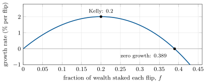
The coin’s Kelly fraction is 0.2: bet 20% of the bankroll on heads each time, for a growth rate of 2.01% a flip. The quadratic form shows the shape of the trade-off (Figure 29.1): growth rises, peaks at $f^*$ , and falls back to zero at about twice $f^*$ ; beyond that, the more one bets, the faster one is ruined, however large the edge. On the coin the growth rate is zero at a stake of 38.9%.

**Figure 29.1.** Growth rate of wealth per flip of the 60% coin at even money, against the fraction of wealth staked. It peaks at the Kelly fraction, 0.2, with 2.01% a flip, and falls to zero at 0.389, about twice Kelly. Data: the chapter’s tutorial.

29.3 Fractional Kelly and risk of ruin

Definition 29.5 (Fractional Kelly, drawdown, risk of ruin)

Fractional Kelly stakes a multiple $c < 1$ of the Kelly fraction. A drawdown is a fall of wealth from its previous peak, measured as a fraction of that peak. The risk of ruin of a staking rule is the probability that wealth ever falls to a given fraction of its starting value.

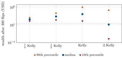
Kelly staking maximises growth, but it is a violent ride: the distribution of wealth after 300 flips is enormously spread (Figure 29.2). Half Kelly gives up a quarter of the growth rate in the quadratic approximation, $g(cf^*) = (2c - c^2)g(f^*)$ , and much of the spread: on the coin, the median after 300 flips is USD 2 279 against 10 504, but the worst tenth of outcomes is better, 251 against 121. Twice Kelly has, to second order, zero growth: half its players end below their stake.

**Figure 29.2.** Wealth after 300 flips of the 60% coin from USD 25 (dashed), uncapped, for four multiples of the Kelly fraction, on a log scale: the 10th, 50th and 90th percentiles of 4 000 simulated players each. Kelly has the highest median; half Kelly the best worst tenth; twice Kelly a median below the stake. Data: the chapter’s tutorial, seeded.

Proposition 29.6 (Risk of falling by a fraction)

In the continuous-time limit of small bets, staking $c$ times the Kelly fraction, the probability that wealth ever falls to a fraction $\alpha$ of its starting value is

P = \alpha^{2/c - 1}.

At full Kelly, the chance of ever halving is one half.

Proof. With stake $c\mu/s^2$ , log wealth is a Brownian motion with drift $m = (c - \tfrac12 c^2)\mu^2/s^2$ and variance $v = c^2\mu^2/s^2$ per unit time. A Brownian motion with drift $m > 0$ and variance $v$ ever falls by $d$ with probability $e^{-2md/v}$ ; with $d = -\ln \alpha$ , $2m/v = 2/c - 1$ . ∎

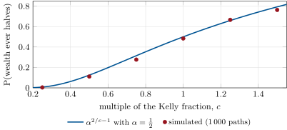
The formula holds up in simulation (Figure 29.3): on a 55% even-money bet over 4 000 bets, the share of paths that ever halved was 48.4% at full Kelly against 50% in theory, 11.1% at half Kelly against 12.5%. Inverting it gives the largest multiple of Kelly for a given tolerance: to keep the chance of ever halving below 10%, $c = 2/(1 + \ln 0.1/\ln 0.5) = 0.46$ . A fall from the peak, which the drawdown measures, recurs over a long enough horizon whatever the fraction: the risk of ruin is the version that has an answer.

Figure 29.3. Probability that wealth ever falls to half its starting value, against the multiple of Kelly staked, on a 55% even-money bet: the continuous-time formula and the share of 1 000 simulated paths of 4 000 bets. Data: the chapter’s tutorial, seeded.

29.4 When the edge itself is uncertain

Everything above assumed the edge known. A trader estimates it, from a backtest or from the strategy’s own history, with an error; and the Kelly fraction is proportional to the edge, so an overestimated edge means overbetting, which costs more growth than the same underbetting.

Proposition 29.7 (Shrinking for estimation error)

Suppose the mean $\mu$ per unit staked is estimated from $n$ trades by $\hat\mu$ , with standard error $s/\sqrt n$ , and the trader stakes $c\hat\mu/s^2$ . In the quadratic approximation the expected growth rate is maximised at

c^* = \frac{\mu^2}{\mu^2 + s^2/n} = \frac{n\,\mathrm{SR}^2}{n\,\mathrm{SR}^2 + 1},

where $\mathrm{SR} = \mu/s$ is the Sharpe ratio per trade; $n\,\mathrm{SR}^2$ is the square of the $t$ -statistic of the edge.

Proof. $E[g] = E[f]\mu - \tfrac12 E[f^2]s^2$ with $f = c\hat\mu/s^2$ , $E[\hat\mu] = \mu$ and $E[\hat\mu^2] = \mu^2 + s^2/n$ , so $E[g] = c\mu^2/s^2 - \tfrac12 c^2(\mu^2 + s^2/n)/s^2$ , maximised at the stated $c$ . ∎

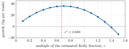
A strategy whose edge has a $t$ -statistic of 1, barely distinguishable from nothing, should stake half of its estimated Kelly fraction; one with a $t$ -statistic of 3, nine tenths. Staking a fraction of Kelly is, in part, this arithmetic (Figure 29.4).

Growth per trade, in basis points, of a trader who estimates the win rate of a 55% even-money bet from 200 trades and then stakes c times the estimated Kelly fraction for 500 trades, averaged over 3 000 repetitions. The best multiple in the simulation is 0.7; the formula gives 0.669. Staking the full estimated Kelly fraction earns 19% less. Data: the chapter’s tutorial, seeded. — **Figure 29.4.** Growth per trade, in basis points, of a trader who estimates the win rate of a 55% even-money bet from 200 trades and then stakes $c$ times the estimated Kelly fraction for 500 trades, averaged over 3 000 repetitions. The best multiple in the simulation is 0.7; the formula gives 0.669. Staking the full estimated Kelly fraction earns 19% less. Data: the chapter’s tutorial, seeded.

The quadratic approximation also hides fat tails: a trade that can lose more than its stake, or a return distribution whose extremes are underestimated, calls for smaller fractions still. And Kelly maximises the growth of one bankroll with no outside constraints; a fund whose investors leave after a 20% loss faces a drawdown constraint that Kelly ignores, and should size with the risk of ruin, not the growth rate.

29.5 Tutorial: repeated bets at several Kelly fractions

Goal. Compute the Kelly fraction and growth rate, simulate repeated bets at several multiples of Kelly, check the risk-of-ruin formula, and find the best multiple when the edge is estimated. End state: Figures 29.1, 29.2, 29.3 and 29.4 and the numbers of the weekend problem.

Kelly and growth, and the simulator.

def kelly_fraction(p: float, b: float = 1.0) -> float:
    """Fraction of wealth to stake on a bet paying b to 1 that wins with probability p (0 if no edge)."""
    return max(p - (1 - p) / b, 0.0)


def growth(f: float, p: float, b: float = 1.0) -> float:
    """Expected log growth of wealth per bet when staking a fraction f."""
    if f >= 1.0:
        return -math.inf
    return p * math.log1p(f * b) + (1 - p) * math.log1p(-f)


def simulate(f: float, p: float, n: int, paths: int, seed: int, b: float = 1.0,
             cap: float = math.inf) -> list[tuple[float, float, float]]:
    """(final wealth, lowest wealth, largest drawdown from a peak) per path, from wealth 1; betting
    stops if wealth reaches `cap`."""
    rng, out = random.Random(seed), []
    for _ in range(paths):
        w, low, peak, dd = 1.0, 1.0, 1.0, 0.0
        for _ in range(n):
            if w >= cap:
                break
            stake = f * w
            w += stake * b if rng.random() < p else -stake
            low, peak = min(low, w), max(peak, w)
            dd = max(dd, 1 - w / peak)
        out.append((min(w, cap), low, dd))
    return out

Listing 29.1. The Kelly fraction, the growth rate and repeated bets. code/firm/sizing/firm_sizing.py

Ruin and estimation error: the drawdown probability, its inverse, and the shrinkage.

def drawdown_probability(c: float, alpha: float) -> float:
    """Probability that wealth ever falls to alpha times its starting value when staking c times
    Kelly (continuous-time approximation)."""
    return alpha ** (2 / c - 1)


def fraction_for_drawdown(alpha: float, delta: float) -> float:
    """Largest multiple of Kelly that keeps the probability of ever falling to alpha of the start
    below delta."""
    return 2 / (1 + math.log(delta) / math.log(alpha))


def shrinkage(n: int, sharpe: float) -> float:
    """Multiple of the estimated Kelly fraction that maximises expected growth when the edge is
    estimated from n trades with per-trade Sharpe ratio `sharpe`."""
    return n * sharpe ** 2 / (n * sharpe ** 2 + 1)


def growth_uncertain(c: float, mu: float, s: float, n: int) -> float:
    """Expected growth per trade (quadratic approximation) when staking c * mu_hat / s^2, mu_hat
    estimated from n trades."""
    se2 = s * s / n
    return c * mu * mu / (s * s) - c * c * (mu * mu + se2) / (2 * s * s)

Listing 29.2. Risk of ruin, the fraction for a tolerance, and shrinkage for an estimated edge. code/firm/sizing/firm_sizing.py

Run sizing_demo.coin_table(), sizing_demo.problem() and fig_sizing.py.

What to change next. Replay the coin with the 250-dollar cap and compare constant fractions with a rule that bets just enough to reach the cap; then give the bets fat-tailed outcomes and find how much the best fraction falls.

29.6 Build: the sizing module

Purpose. Every strategy of the miniature firm is sized here: a fraction of capital from its estimated edge and risk, cut for estimation error and for the firm’s tolerance of drawdowns.

Interface. kelly_fraction(p, b); growth(f, p, b); simulate(f, p, n, paths, seed, b, cap); drawdown_probability(c, alpha); fraction_for_drawdown(alpha, delta); shrinkage(n, sharpe); growth_uncertain(c, mu, s, n).

Rules. Wealth multiplicative, stakes a fixed fraction of current wealth; the risk of ruin in its continuous-time form; the shrinkage in the quadratic approximation; seeded simulations.

Acceptance tests. code/firm/sizing/tests/: Kelly maximises growth, twice Kelly has about zero growth; the ruin formula and its inverse agree; simulated falls to half match the formula; the shrinkage maximises the expected growth.

Stretch. Kelly for several correlated strategies (the fraction becomes $\Sigma^{-1}\mu$ ); fat tails; sizing under a hard drawdown limit; Bayesian updating of the edge as trades arrive (One Quant Book 4).

Sources and further reading

V. Haghani and R. Dewey, “Rational decision-making under uncertainty: observed betting patterns on a biased coin”, October 2016.
J. L. Kelly, “A new interpretation of information rate”, Bell System Technical Journal, 1956.

29.7 Exercises

Exercise 29.1 ★

A bet pays 2 to 1 and wins with probability 0.4. What are its edge and its Kelly fraction?

Solution

Solution of Exercise 29.1.

Edge $0.4 \times 2 - 0.6 = 0.2$ per unit staked; Kelly fraction $0.2/2 = 0.1$ .

Exercise 29.2 ★

Why is the expected wealth after 300 flips a poor guide to what a player ends with?

Solution

Solution of Exercise 29.2.

It is dominated by a few enormously lucky paths: the expected wealth grows like $1.04^{300}$ while almost every player’s wealth grows like $e^{300g}$ , which is far smaller. The median, or the growth rate, describes what a typical player gets.

Exercise 29.3 ★

What fraction of the full Kelly growth rate does half Kelly keep, in the quadratic approximation? And a quarter Kelly?

Solution

Solution of Exercise 29.3.

$2c - c^2$ : 75% at half Kelly, 43.75% at a quarter.

Exercise 29.4 ★★

At full Kelly, what is the probability of ever falling to 20% of starting wealth? At half Kelly?

Solution

Solution of Exercise 29.4.

$0.2^{2/1 - 1} = 20\%$ at full Kelly; $0.2^{3} = 0.8\%$ at half Kelly.

Exercise 29.5 ★★

A fund’s investors leave if it ever loses 20% of its starting capital, and it accepts a 10% chance of that. What multiple of Kelly should it use?

Solution

Solution of Exercise 29.5.

$c = 2/(1 + \ln 0.1/\ln 0.8) = 0.18$ : less than a fifth of Kelly.

Exercise 29.6 ★★

An edge is estimated with a $t$ -statistic of 2. What multiple of the estimated Kelly fraction maximises expected growth?

Solution

Solution of Exercise 29.6.

$t^2/(t^2 + 1) = 4/5 = 0.8$ .

Exercise 29.7 ★★★

Coding. With simulate and a cap of ten times the stake, estimate the share of players who reach the cap in 300 flips of the 60% coin at half Kelly and at Kelly, and compare with the 95% quoted by Haghani and Dewey.

Solution

Solution of Exercise 29.7.

About 94% at half Kelly and at Kelly (94.2% and 93.7% in 4 000 seeded players), close to the 95% the authors quote for constant fractions of 10 to 20%.

Exercise 29.8 ★★★

Find the flaw. “Our backtest shows an edge with a Sharpe ratio of 0.1 per trade over 200 trades, so we stake the full Kelly fraction: it maximises growth.” Correct it.

Solution

Solution of Exercise 29.8.

With a Sharpe ratio of 0.1 over 200 trades the edge has a $t$ -statistic of about 1.4: it is uncertain, and staking the full estimated Kelly fraction overbets whenever the estimate is high. The expected growth is maximised at about two thirds of the estimated fraction, and full Kelly also carries a 50% chance of ever halving the capital.

29.8 Problem: The Uncertain Edge

Problem 29.1

Weekend problem — how much of Kelly to stake

A trader has a signal that, it believes, wins 55% of the time on even-money trades. It has seen 200 trades, and will size the next 500 as a fraction of capital.

Part I — The known edge.

If the win rate is exactly 55%, what are the edge, the Kelly fraction and the growth rate per trade?
What are the mean and standard deviation of the profit per unit staked, and the Sharpe ratio per trade?
At full Kelly, what is the probability of ever halving the capital?
What multiple of Kelly keeps that probability below 10%?
Why does staking twice Kelly destroy the edge?

Part II — The estimate.

What is the standard error of the win-rate edge estimated from 200 trades, and its $t$ -statistic?
What multiple of the estimated Kelly fraction maximises expected growth?
What does the simulation give?
How much growth does staking the full estimated Kelly fraction lose against the best multiple?
At the best multiple, what is the probability of ever halving?

Part III — Robustness.

How does the best multiple change with 50 trades of history? With 2 000?
Why is overbetting worse than underbetting by the same amount?
What would fat tails do to the best fraction?
How would you combine this shrinkage with a drawdown limit?
What does the coin experiment say about sizing in practice?

Part IV — Judgement.

Why might a firm size strategies at a quarter Kelly or less?
How would you update the fraction as new trades arrive?
When is the Kelly framework the wrong one?
State the named result: the best multiple of Kelly when the edge is estimated from 200 trades.
In one sentence: why stake less than Kelly?

Solution

Solution of Problem 29.1.

1. Edge 0.1 per unit staked, Kelly fraction 0.1, growth 0.501% per trade. 2. Mean 0.1, standard deviation 0.995, Sharpe ratio 0.1005 per trade. 3. 50%. 4. 0.46 of Kelly. 5. To second order the growth rate at twice Kelly is zero: the gain from the edge is exactly offset by the variance drag of the larger stakes. 6. The mean is estimated with a standard error of 0.0704; $t = 1.42$ . 7. $c^* = 0.669$ . 8. 0.7, the best of the multiples tried, in steps of 0.1. 9. 19%: 29.1 against 35.9 basis points a trade. 10. $0.5^{2/0.669 - 1} = 25\%$ . 11. With 50 trades, 0.34; with 2 000, 0.95. 12. Growth falls quadratically around the Kelly fraction but the drag grows with the square of the stake, and an overestimated edge raises the stake; the losses from overbetting include a real chance of ruin, those from underbetting only slower growth. 13. Lower it: losses larger than the variance suggests make large stakes costlier than the quadratic approximation shows. 14. Take the smaller of the shrunk Kelly multiple and the multiple that keeps the risk of ruin within the tolerance. 15. That people with a clear edge, when free to size, overbet and bet erratically: a sizing rule decided in advance protects the edge from the trader. 16. Because edges are estimated with error and decay, returns have fat tails, strategies are correlated, and investors and counterparties impose drawdown limits long before ruin. 17. Bayesian updating of the edge’s estimate and its uncertainty after each trade, recomputing the shrunk fraction, with limits on how fast it may change. 18. When the goal is not long-run growth of one bankroll: a fixed horizon, a cap on payout, a hard drawdown limit, or utility with more risk aversion than the logarithm. 19. Named result: the uncertain edge: with the edge estimated from 200 trades at a Sharpe ratio of 0.1, the best stake is two thirds of the estimated Kelly fraction (0.669 by the formula, 0.7 in simulation), which earns 19% more growth than full Kelly. 20. Because the edge is an estimate, and overbetting it costs more than underbetting.

29.9 Interview questions

Interview question 29.1 ★ trader, researcher

A coin lands heads 60% of the time and pays even money. How much of your wealth do you bet, and why?

Solution

Solution of Interview question 29.1.

Twenty per cent: the Kelly fraction $p - q/b = 0.6 - 0.4$ , which maximises the long-run growth rate at about 2% a flip. Betting more raises the variance drag faster than the gain; above about 39% wealth shrinks in the long run.

What the interviewer is looking for: edge over odds, and why not more.

Interview question 29.2 ★ trader

What is the difference between maximising expected wealth and maximising expected log wealth?

Solution

Solution of Interview question 29.2.

Expected wealth rewards staking everything, since a few huge outcomes dominate it; expected log wealth is the growth rate that almost every path achieves over many bets, and it penalises variance. Maximising it gives Kelly; maximising the mean gives ruin.

What the interviewer is looking for: typical versus average outcome.

Interview question 29.3 ★★ researcher

Derive the Kelly fraction for a continuous return with mean $\mu$ and variance $\sigma^2$ .

Solution

Solution of Interview question 29.3.

Over a short period $dt$ , the log return of wealth with fraction $f$ in the asset (and the rest at zero rate) has mean $f\mu\,dt - \tfrac12 f^2\sigma^2 dt$ ; maximising gives $f^* = \mu/\sigma^2$ and growth $\mu^2/(2\sigma^2)$ , half the squared Sharpe ratio.

What the interviewer is looking for: Ito’s correction and the quadratic.

Interview question 29.4 ★★ researcher, risk

Why do practitioners use fractional Kelly?

Solution

Solution of Interview question 29.4.

Half Kelly keeps three quarters of the growth with half the volatility; it guards against overestimated edges and fat tails; and it keeps drawdowns within what investors and risk limits tolerate: the chance of ever halving falls from 50% to 12.5%.

What the interviewer is looking for: growth versus risk, and estimation error.

Interview question 29.5 ★★ trader, researcher

You have two uncorrelated strategies with Sharpe ratios 1 and 2. How do you split capital between them?

Solution

Solution of Interview question 29.5.

The Kelly weights are $\mu_i/\sigma_i^2 = \mathrm{SR}_i/\sigma_i$ : with equal volatilities, twice the capital to the Sharpe-2 strategy; in general in proportion to Sharpe ratio over volatility, then scaled down for estimation error and limits.

What the interviewer is looking for: $\Sigma^{-1}\mu$ with no correlation.

Interview question 29.6 ★★★ developer

Design a sizing service that sets each strategy’s capital daily from its live performance, with limits.

Solution

Solution of Interview question 29.6.

Each day, estimate each strategy’s edge and risk from its live and backtest history with their uncertainty; compute the shrunk Kelly fraction, cap it by the drawdown rule, by correlations with the other strategies and by capacity; smooth changes; publish the allocations with their inputs; override on breaches; and log everything for review.

What the interviewer is looking for: estimation, shrinkage, limits, smoothing, audit.

Terms defined in this chapter

See all 2333 terms in the glossary