University Mathematics — Year 2 · Bachelor Year 2

10Sequences and Series of Functions

When functions converge to a function, which properties survive the passage to the limit? Pointwise convergence preserves almost nothing; uniform convergence — convergence in the sup norm — preserves continuity, integrals on segments and, with one twist, derivatives. This chapter proves the three transfer theorems, their series versions, and crowns them with the Weierstrass approximation theorem, proved by Bernstein’s beautiful probabilistic polynomials.

10.1 Pointwise and uniform convergence

Definition 10.1

Let $f_n, f \colon X \to \R$ (or $\C$ , or a normed space), $X$ any set. $(f_n)$ converges to $f$ pointwise when $f_n(x) \to f(x)$ for every $x$ ; uniformly when

\norm{f_n - f}_\infty = \sup_{x \in X}\, \abs{f_n(x) - f(x)} \xrightarrow[n \to \infty]{} 0 .

Uniform implies pointwise; on $C(\intcc{a}{b})$ , uniform convergence is exactly convergence in the Banach space $\bigl(C(\intcc{a}{b}), \norm\cdot_\infty\bigr)$ of Chapter 5.

Example 10.2

On $\intcc{0}{1}$ , $f_n(x) = x^n$ converges pointwise to the discontinuous limit $f = \mathbf{1}_{\{1\}}$ ; the convergence is not uniform: $\norm{f_n - f}_\infty \geq f_n\bigl(1 - \tfrac1n\bigr) = (1 - \tfrac1n)^n \to \eu^{-1} \neq 0$ . On $\intcc{0}{a}$ with $a < 1$ it is uniform ( $\sup = a^n \to 0$ ): uniformity is a property of the domain as much as of the sequence.

The sequence xn on [0, 1]: the graphs sag toward 0 but all must climb to 1 at x = 1 — the sup distance to the discontinuous pointwise limit never shrinks below a constant. — The sequence $x^n$ on $\intcc{0}{1}$ : the graphs sag toward $0$ but all must climb to $1$ at $x = 1$ — the sup distance to the discontinuous pointwise limit never shrinks below a constant.

Example 10.3 (Two limits that refuse to commute)

The whole chapter is about interchanging limits, so here is the smallest possible failure. Let $a_{n,m} = \dfrac{n}{n+m}$ for $n, m \geq 1$ . Then

\lim_{m\to\infty}\Bigl(\lim_{n\to\infty}a_{n,m}\Bigr) = \lim_{m\to\infty} 1 = 1, \qquad \lim_{n\to\infty}\Bigl(\lim_{m\to\infty}a_{n,m}\Bigr) = \lim_{n\to\infty} 0 = 0 :

both iterated limits exist and they differ. Every transfer theorem of this chapter is a licence to commute two limits — $\lim_n$ with $\lim_{x\to a}$ (continuity), with $\int$ (integration), with $\frac{\dd}{\dd x}$ (differentiation) — and uniform convergence is precisely the fee that makes the commutation legal. Closing insight: whenever a “proof” silently swaps two limit operations, this two-line array is the counterexample to hold against it; the sliding bumps of Exercise 10.2 are the same phenomenon wearing an integral sign.

10.2 The three transfer theorems

Theorem 10.4 (Continuity)

If each $f_n$ is continuous at $a$ and $f_n \to f$ uniformly on a neighborhood of $a$ , then $f$ is continuous at $a$ . A uniform limit of continuous functions is continuous.

Proof. The $3\varepsilon$ argument already used in Theorem 4.9: pick $n$ with $\norm{f_n - f}_\infty \leq \varepsilon$ , then $\delta$ from continuity of $f_n$ at $a$ ; for $\abs{x - a} \leq \delta$ ,

\abs{f(x) - f(a)} \leq \abs{f(x) - f_n(x)} + \abs{f_n(x) - f_n(a)} + \abs{f_n(a) - f(a)} \leq 3\varepsilon . \qedhere

∎

Example 10.5 (Uniformity fails exactly where the limit breaks)

On $\intcc{0}{2}$ , let $f_n(x) = \dfrac{x^n}{1 + x^n}$ . The pointwise limit is a three-piece function:

f(x) = \begin{cases} 0 & 0 \leq x < 1,\\[2pt] \tfrac12 & x = 1,\\[2pt] 1 & 1 < x \leq 2, \end{cases}

discontinuous at $1$ , so by Theorem 10.4 the convergence cannot be uniform on $\intcc{0}{2}$ . On the closed pieces avoiding the threshold it is: for $0 \leq x \leq a < 1$ ,

\sup_{\intcc{0}{a}}\abs{f_n - 0} = \frac{a^n}{1 + a^n} \leq a^n \to 0 ,

and for $1 < b \leq x \leq 2$ ,

\sup_{\intcc{b}{2}}\abs{f_n - 1} = \frac{1}{1 + b^n} \leq b^{-n} \to 0 ,

both suprema computed by monotonicity of $u \mapsto \frac{u}{1+u}$ and of $x \mapsto x^n$ . Closing insight: the failure of uniformity is localized at the discontinuity of the limit — the same geometry as Example 10.2, and the reason the “uniform on every segment inside” discipline recurs all chapter long.

Theorem 10.6 (Integration on a segment)

If $f_n \to f$ uniformly on $\intcc{a}{b}$ , with $f_n$ piecewise continuous ( $f$ likewise), then

\int_a^b f_n \longrightarrow \int_a^b f .

Proof. Linearity and the triangle inequality for integrals give

\Bigl|\int_a^b f_n - \int_a^b f\Bigr| = \Bigl|\int_a^b (f_n - f)\Bigr| \leq \int_a^b\abs{f_n - f} \leq (b - a)\,\norm{f_n - f}_\infty \longrightarrow 0 .

The length factor $(b - a)$ is where compactness of the segment enters: on non-compact intervals the same estimate produces the useless bound $\infty\cdot0$ , and the conclusion genuinely fails without domination — the flat bumps $f_n = \frac1n\mathbf 1_{\intcc{0}{n}}$ converge uniformly to $0$ on $\intco{0}{\infty}$ yet keep $\int f_n = 1$ (pitfalls remark below), and the sliding bumps of Chapter 9’s remark do the same with pointwise convergence; uniform convergence controls heights, never widths. ∎

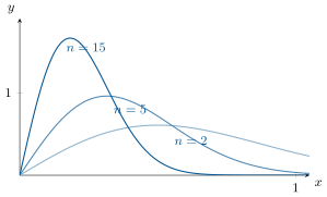
The bumps g_n(x) = nx\, -nx2 of : they converge to 0 at every point, but the peaks (height √n/(2 ), drifting toward 0) grow without bound — pointwise convergence with g_n_∈fty ∈fty, and ∈t_01 g_n 1/2 ≠ 0: the mass hides under the moving peak. — The bumps $g_n(x) = nx\,\eu^{-nx^2}$ of Exercise 10.1: they converge to $0$ at every point, but the peaks (height $\sim\sqrt{n/(2\eu)}$ , drifting toward $0$ ) grow without bound — pointwise convergence with $\norm{g_n}_\infty \to \infty$ , and $\int_0^1 g_n \to \frac12 \neq 0$ : the mass hides under the moving peak.

Theorem 10.7 (Differentiation)

Let $f_n$ be $C^1$ on an interval $I$ , with: $(f_n')$ converging uniformly on $I$ (or on every segment of $I$ ) to some $g$ , and $(f_n(x_0))$ converging at one point $x_0$ . Then $(f_n)$ converges (uniformly on segments) to a $C^1$ function $f$ , and $f' = g$ : one may differentiate the limit.

Proof. Define $f(x) = \lim f_n(x_0) + \int_{x_0}^x g$ : legitimate, $g$ being continuous — indeed $g$ is the uniform limit on segments of the continuous $f_n'$ , so Theorem 10.4 applies, and the integral of a continuous function is well defined with, by the fundamental theorem of calculus,

f'(x) = g(x) \qquad (x \in I) :

the candidate limit is $C^1$ with the right derivative by construction, before any convergence is proved. By the fundamental theorem again, $f_n(x) = f_n(x_0) + \int_{x_0}^x f_n'$ ; subtracting,

\abs{f_n(x) - f(x)} \leq \abs{f_n(x_0) - \lim f_n(x_0)} + \abs{x - x_0}\,\norm{f_n' - g}_{\infty} ,

which tends to $0$ uniformly on every segment. And $f$ is $C^1$ with $f' = g$ by construction. ∎

Example 10.8 (Why the hypothesis sits on the derivatives)

Let $F_n(x) = \sqrt{x^2 + \frac1n}$ on $\R$ . Each $F_n$ is $C^1$ (indeed $C^\infty$ ), and the convergence to $\abs x$ is uniform on all of $\R$ :

0 \leq F_n(x) - \abs x = \frac{(x^2 + \frac1n) - x^2}{\sqrt{x^2+\frac1n} + \abs x} = \frac{1/n}{\sqrt{x^2 + \frac1n} + \abs x} \leq \frac{1/n}{1/\sqrt n} = \frac{1}{\sqrt n} .

Yet the limit $\abs x$ is not differentiable at $0$ : uniform convergence of the functions, however fast, transfers no differentiability. The failure is visible on the derivatives:

F_n'(x) = \frac{x}{\sqrt{x^2 + \frac1n}} \longrightarrow \begin{cases} 1 & x > 0,\\ 0 & x = 0,\\ -1 & x < 0, \end{cases}

a discontinuous pointwise limit, so $(F_n')$ cannot converge uniformly near $0$ (Theorem 10.4 again). Closing insight: Theorem 10.7 deliberately assumes uniform convergence of the $f_n'$ , not of the $f_n$ — this example is the reason.

10.3 Series of functions

Definition 10.9

A series of functions $\sum u_n$ converges pointwise/uniformly when its partial sums do. It converges normally (on $X$ ) when $\sum \norm{u_n}_\infty < \infty$ . Normal convergence implies uniform convergence (in the Banach space of bounded functions: Theorem 5.21), which implies pointwise; both implications are strict.

Example 10.10 (One series, three verdicts)

Take $u_n(x) = \frac{x^n}{n}$ on $\intco{0}{1}$ . Pointwise: converges for every $x \in \intco01$ (comparison with the geometric series). Normal on $\intcc{0}{a}$ , $a < 1$ : $\norm{u_n}_{\infty,\intcc0a} = \frac{a^n}{n}$ , summable. Not normal on $\intco{0}{1}$ : $\norm{u_n}_{\infty,\intco01} = \frac1n$ , and $\sum\frac1n$ diverges. Not even uniform on $\intco{0}{1}$ : the remainder resists near $1$ ,

R_N(x) = \sum_{n>N}\frac{x^n}{n} \geq \sum_{n=N+1}^{2N}\frac{x^n}{n} \geq \frac{N\,x^{2N}}{2N} = \frac{x^{2N}}{2} \xrightarrow[x\to1^-]{} \frac12 ,

so $\sup_{\intco01}\abs{R_N} \geq \frac12$ for every $N$ . Closing insight: all four verdicts coexist peacefully — the sum $-\ln(1-x)$ is continuous on $\intco{0}{1}$ because continuity only needs uniformity near each point, i.e. on the segments $\intcc0a$ ; blowing up at the edge is the sum’s right.

Theorem 10.11 (Transfer for series)

If $\sum u_n$ converges uniformly (e.g. normally) on the relevant set: continuity of all $u_n$ at $a$ passes to the sum; integration on a segment can be done term by term; and if $\sum u_n(x_0)$ converges while $\sum u_n'$ converges uniformly on segments, the sum is $C^1$ with derivative $\sum u_n'$ .

Proof. Everything is the corresponding theorem applied to the partial sums $S_N = \sum_{n\leq N}u_n$ , which are finite sums of functions with the relevant regularity. Continuity: each $S_N$ is continuous at $a$ and $S_N \to \sum u_n$ uniformly: Theorem 10.4. Integration: on the segment,

\int_a^b \sum_{n\geq0} u_n = \lim_N \int_a^b S_N = \lim_N \sum_{n=0}^{N}\int_a^b u_n = \sum_{n\geq0}\int_a^b u_n

by Theorem 10.6 (first equality) and linearity of the integral (second). Differentiation: the $S_N$ are $C^1$ , $S_N(x_0)$ converges, and $S_N' = \sum_{n\leq N}u_n'$ converges uniformly on segments: Theorem 10.7 gives that the sum is $C^1$ with derivative $\lim S_N' = \sum u_n'$ . ∎

Remark 10.12 (Common pitfalls)

Four traps, all seen in examination copies. (i) Half-checked suprema: evaluating $f_n$ along a well-chosen sequence $x_n$ only bounds $\norm{f_n - f}_\infty$ from below — enough to disprove uniformity (as in Example 10.2), never to prove it; to prove it, bound the sup by a computation valid for all $x$ . (ii) Uniformity on the wrong set: normal or uniform convergence often holds on every $\intcc{-a}{a}$ or $\intco\delta\infty$ but fails on the open union; that is no obstacle — continuity and differentiability are local, so the segment-by-segment discipline of Example 10.13 gives them on the whole open set. (iii) Integrating over non-segments: Theorem 10.6 is a statement about segments; on $\intco0\infty$ , uniform convergence does not prevent mass from escaping to infinity ( $f_n = \frac1n\mathbf 1_{\intcc{0}{n}}$ converges uniformly to $0$ , with $\int f_n = 1$ ) — use dominated convergence there. (iv) Differentiating the limit: Example 10.8; the derivative hypothesis is on $(f_n')$ , and no rate of convergence of $(f_n)$ can replace it.

Example 10.13 (The Riemann $\zeta$ function)

$\zeta(s) = \sum_{n\geq1} n^{-s}$ converges normally on every half-line $\intco{a}{+\infty}$ , $a > 1$ ( $\norm{n^{-s}}_\infty = n^{-a}$ , summable): $\zeta$ is continuous on $\intoo{1}{+\infty}$ ; differentiating termwise (the derived series $\sum -\ln n\; n^{-s}$ also converges normally on $\intco{a}{\infty}$ ), $\zeta$ is $C^1$ — and, iterating, $C^\infty$ — with $\zeta'(s) = -\sum \frac{\ln n}{n^s}$ . Note the discipline: normal convergence is checked on sub-half-lines, never on the open $\intoo{1}{\infty}$ itself, where it fails.

Example 10.14 (A logarithmic series, worked to the end)

Let $F(x) = \sum_{n\geq1} \frac{\eu^{-nx}}{n}$ on $\intoo{0}{\infty}$ . Each term is bounded on $\intco{\delta} \infty$ by $\frac{\eu^{-n\delta}}{n} \leq \eu^{-n\delta}$ , a convergent geometric series: normal convergence on every $\intco\delta\infty$ , so $F$ is continuous on $\intoo{0}{\infty}$ . The derived series $\sum -\eu^{-nx}$ is likewise normally convergent on $\intco\delta\infty$ ( $\norm{\eu^{-nx}}_{\infty,\intco\delta\infty} = \eu^{-n\delta}$ ), so $F$ is $C^1$ with a geometric derivative:

F'(x) = -\sum_{n\geq1}\eu^{-nx} = \frac{-\eu^{-x}}{1 - \eu^{-x}} = \frac{-1}{\eu^{x} - 1} .

Iterating, $F$ is $C^\infty$ . Integrating $F'$ (both $F$ and $x \mapsto -\ln(1 - \eu^{-x})$ vanish at $+\infty$ and have the same derivative on $\intoo0\infty$ ):

F(x) = -\ln\bigl(1 - \eu^{-x}\bigr),

the logarithmic series at $t = \eu^{-x}$ . Closing insight: as $x \to 0^+$ , $F(x) = -\ln(x + O(x^2)) = \ln\frac1x + O(x)$ — the series diverges logarithmically at the boundary, exactly like the harmonic series it becomes at $x = 0$ ; normal convergence on $\intco\delta\infty$ but not on $\intoo0\infty$ is the symptom.

Method 10.15 (Proving or disproving uniform convergence)

For $f_n \to f$ pointwise on $X$ :

Compute or bound $\norm{f_n - f}_\infty$ : study the function $x \mapsto \abs{f_n(x) - f(x)}$ (derivative, monotonicity) to locate its maximum; a bound valid for all $x$ that tends to $0$ proves uniformity.
To disprove: exhibit points $x_n$ with $\abs{f_n(x_n) - f(x_n)} \not\to 0$ (often $x_n$ tracks the moving bump, as in Exercise 10.1); or invoke a transfer theorem in contrapositive — a discontinuous limit of continuous functions (Example 10.5), or $\int f_n \not\to \int f$ on a segment.
For series, try normal convergence first ( $\sum\sup\abs{u_n} < \infty$ ); if it fails globally, test it on the sub-segments that matter (Example 10.10); if it fails everywhere, uniform convergence may still hold via the alternating remainder bound (Exercise 10.4) or summation by parts.

10.4 The Weierstrass approximation theorem

Theorem 10.16 (Weierstrass, via Bernstein)

Every continuous $f \colon \intcc{0}{1} \to \R$ is a uniform limit of polynomials — explicitly, of its Bernstein polynomials

B_n(f)(x) = \sum_{k=0}^{n} f\Bigl(\frac kn\Bigr)\binom nk x^k (1-x)^{n-k} .

Proof. Fix $x \in \intcc{0}{1}$ and set $p_k(x) = \binom nk x^k(1 - x)^{n-k}$ . Three binomial identities, obtained by evaluating $(x + y)^n$ and its two $x$ -derivatives at $y = 1 - x$ :

\sum_k p_k = 1, \qquad \sum_k k\,p_k = nx, \qquad \sum_k k(k-1) p_k = n(n-1)x^2 .

In detail: $(x+y)^n = \sum_k\binom nk x^ky^{n-k}$ at $y = 1-x$ is the first; differentiating in $x$ ,

n(x+y)^{n-1} = \sum_k k\binom nk x^{k-1}y^{n-k} ,

then multiplying by $x$ and setting $y = 1 - x$ gives the second; differentiating twice and multiplying by $x^2$ gives the third. Expanding $(k - nx)^2 = k(k-1) + k(1 - 2nx) + n^2x^2$ and combining the three:

\sum_k (k - nx)^2 p_k = n(n-1)x^2 + nx(1 - 2nx) + n^2x^2 = nx(1 - x) \leq \frac n4 ,

the variance identity.

Now estimate, using $\sum p_k = 1$ :

\abs{B_n(f)(x) - f(x)} \leq \sum_{k} \Bigl| f\Bigl(\frac kn\Bigr) - f(x)\Bigr|\, p_k(x) = \Sigma_{\text{near}} + \Sigma_{\text{far}} ,

splitting according to $\abs{\frac kn - x} \leq \delta$ or not. Given $\varepsilon > 0$ , uniform continuity of $f$ (Heine) provides $\delta$ with $\Sigma_{\text{near}} \leq \varepsilon$ . For the far sum, with $M = \norm f_\infty$ : by the variance identity and Chebyshev’s counting trick,

\Sigma_{\text{far}} \leq 2M \sum_{\abs{k - nx} > n\delta} p_k \leq 2M\,\frac{\sum_k (k - nx)^2 p_k}{n^2\delta^2} \leq \frac{2M}{4 n \delta^2} \cdot 1 = \frac{M}{2n\delta^2} \xrightarrow[n\to\infty]{} 0 ,

uniformly in $x$ . So $\norm{B_n(f) - f}_\infty \leq \varepsilon + \frac{M}{2n\delta^2} \leq 2\varepsilon$ for large $n$ . ∎

Remark 10.17

By affine substitution the theorem holds on any segment $\intcc{a}{b}$ . It fails on $\R$ (a uniform limit of polynomials on $\R$ is a polynomial: Exercise 10.8). The probabilistic reading — $B_n(f)(x)$ is the expected value of $f$ at a binomial average, and the variance bound is Chebyshev’s inequality — is made honest in Chapter 23.

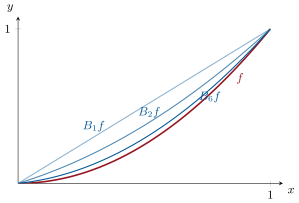
Bernstein approximation of f(x) = x2 (red), using the exact formula B_nf = x2 + x(1-x)/n of : B_1f is the chord, and each doubling of n halves the gap. Reliable but slow — the 1n saturation that Voronovskaya’s theorem (weekend problem) makes exact. — Bernstein approximation of $f(x) = x^2$ (red), using the exact formula $B_nf = x^2 + \frac{x(1-x)}{n}$ of Exercise 10.7: $B_1f$ is the chord, and each doubling of $n$ halves the gap. Reliable but slow — the $\frac1n$ saturation that Voronovskaya’s theorem (weekend problem) makes exact.

Remark 10.18 (Where this is used)

Weierstrass approximation is the density theorem of classical analysis: it makes $C(\intcc ab)$ separable, lets one check integral identities on polynomials only (moment problems), and underlies the trigonometric version proved in the Fourier chapter via Fejér’s kernel. The weekend problem of this chapter extracts the quantitative content of Bernstein’s proof — convergence rates governed by the modulus of continuity — and then isolates what really made it work, in Korovkin’s theorem: positivity plus three test functions. The Year 3 volume generalizes the density statement to arbitrary subalgebras (Stone–Weierstrass) and to compact spaces.

Example 10.19 (Polygonal approximation, with a rate)

For $L$ -Lipschitz $f$ on $\intcc{0}{1}$ , let $I_nf$ be the piecewise-affine interpolant at the nodes $\frac kn$ . On a cell $\intcc{\frac kn}{\frac{k+1}n}$ , both $f(x)$ and $I_nf(x)$ lie between the extreme values that an $L$ -Lipschitz function can take given the two nodal values, so for $x$ in the cell, writing $x_k = \frac kn$ :

\abs{I_nf(x) - f(x)} \leq \abs{I_nf(x) - f(x_k)} + \abs{f(x_k) - f(x)} \leq L\,\abs{x - x_k} + L\,\abs{x - x_k} \leq \frac{2L}{n}

(the interpolant is itself $L$ -Lipschitz on the cell: its slope is a difference quotient of $f$ ). Hence $\norm{I_nf - f}_\infty \leq \frac{2L}{n}$ : polygonal approximation of Lipschitz functions converges at speed $\frac1n$ — faster than Bernstein’s $\frac{1}{\sqrt n}$ for the same class (weekend problem, Part II). Closing insight: the polygon interpolates but is not smooth, Bernstein is smooth but slow; there is no free lunch between regularity of the approximant and speed — a trade-off made precise by the saturation results of the weekend problem.

Remark 10.20 (Perspectives within this volume)

Uniform convergence is this book’s workhorse from here on. The power-series chapter runs entirely on normal convergence on compact subdisks — every term-by-term theorem there is a special case of this chapter’s transfer theorems. The Fourier chapter lives one floor up: its partial sums $S_N$ fail exactly where this chapter warns they might (pointwise but not uniform at jumps), and its Fejér means succeed by the same $3\varepsilon$ mechanics that proved Theorem 10.4. The differential-equations chapter defines $\eu^{tA}$ by a normally convergent series and differentiates it termwise — literally Theorem 10.11 applied to matrix entries. When in doubt later in the book about “why can we do this”, the answer is usually a theorem of this chapter.

10.5 Exercises

Exercise 10.1 ★

Study the pointwise and uniform convergence on $\intcc{0}{1}$ , then on $\intcc{0}{a}$ ( $a < 1$ ) or $\intco{\delta}{1}$ as relevant, of:

f_n(x) = \frac{x}{1 + nx}, \qquad g_n(x) = n x\,\eu^{-n x^2}, \qquad h_n(x) = x^n(1 - x^n).

Solution

Solution of Exercise 10.1.

$f_n(x) = \frac{x}{1 + nx}$ : pointwise limit $0$ on $\intcc{0}{1}$ . Uniformly: $f_n$ increases on $\intcc{0}{1}$ (derivative $\frac{1}{(1+nx)^2} > 0$ ), so $\norm{f_n}_\infty = f_n(1) = \frac{1}{1+n} \to 0$ : uniform on $\intcc{0}{1}$ .

$g_n(x) = nx\,\eu^{-nx^2}$ : pointwise limit $0$ (exponential beats). Sup: $g_n' = n\eu^{-nx^2}(1 - 2nx^2)$ vanishes at $x_n = \frac{1}{\sqrt{2n}}$ , where $g_n(x_n) = \sqrt{\frac n2}\,\eu^{-1/2} \to \infty$ : not uniform on $\intcc{0}{1}$ — but uniform on $\intco{\delta}{1}$ , since there $g_n(x) \leq n\,\eu^{-n\delta^2} \to 0$ .

$h_n(x) = x^n(1 - x^n)$ : pointwise limit $0$ on $\intcc{0}{1}$ (both factors; at $x = 1$ , $h_n = 0$ ). Sup: with $u = x^n \in \intcc{0}{1}$ , $u(1-u) \leq \frac14$ attained at $u = \frac12$ , i.e. $x = 2^{-1/n} \in \intoo{0}{1}$ : $\norm{h_n}_\infty = \frac14 \not\to 0$ : not uniform on $\intcc{0}{1}$ ; uniform on $\intcc{0}{a}$ ( $\sup \leq a^n \to 0$ ).

Exercise 10.2 ★

Prove that $\displaystyle\int_0^1 g_n \not\to \int_0^1 \lim g_n$ for the $g_n$ of Exercise 10.1, and reconcile with Theorem 10.6.

Solution

Solution of Exercise 10.2.

$\int_0^1 nx\,\eu^{-nx^2}\dd x = \bigl[-\tfrac12 \eu^{-nx^2}\bigr]_0^1 = \frac{1 - \eu^{-n}}{2} \to \frac12$ , while $\int_0^1 \lim g_n = 0$ . No contradiction: Theorem 10.6 requires uniform convergence on the segment, which fails here (the bump of height $\sim\sqrt n$ slides toward $0$ ).

Exercise 10.3 ★

Prove that $S(x) = \sum_{n\geq1} \dfrac{x^n}{n^2}$ is continuous on $\intcc{-1}{1}$ , and that $S$ is $C^1$ on $\intoo{-1}{1}$ with $S'(x) = -\frac{\ln(1-x)}{x}$ for $0 < \abs x < 1$ .

Solution

Solution of Exercise 10.3.

Normal convergence on $\intcc{-1}{1}$ : $\norm{x^n/n^2}_\infty = \frac{1}{n^2}$ , summable: $S$ is continuous there (Theorem 10.11).

Derivative: the derived series $\sum \frac{x^{n-1}}{n}$ converges normally on every $\intcc{-a}{a}$ , $a < 1$ ( $\sup = \frac{a^{n-1}}{n}$ ): $S$ is $C^1$ on $\intoo{-1}{1}$ with

S'(x) = \sum_{n\geq1} \frac{x^{n-1}}{n} = \frac1x \sum_{n\geq1} \frac{x^n}{n} = -\frac{\ln(1 - x)}{x} \qquad (0 < \abs x < 1),

the last identity being the Year 1 logarithmic series (re-derived honestly in Chapter 11).

Exercise 10.4 ★★

Let $F(x) = \sum_{n \geq 0} \dfrac{(-1)^n}{n + x}$ on $\intoo{0}{+\infty}$ . Prove uniform (not normal) convergence on $\intco{\delta}{\infty}$ via the alternating series remainder bound, continuity, and the functional equation $F(x) + F(x + 1) = \frac1x$ .

Solution

Solution of Exercise 10.4.

For fixed $x > 0$ the series is alternating with $\frac{1}{n + x} \downarrow 0$ : pointwise convergence, and the remainder bound $\abs{R_N(x)} \leq \frac{1}{N + 1 + x} \leq \frac{1}{N+1}$ is uniform on $\intco{\delta}{\infty}$ (indeed on $\intoo{0}{\infty}$ ): uniform convergence. (Not normal: $\norm{\frac{(-1)^n}{n+x}}_\infty = \frac{1}{n + \delta}$ , divergent.) Continuity follows from Theorem 10.11.

Functional equation: reindex $F(x + 1)$ with $m = n + 1$ :

F(x+1) = \sum_{n\geq0} \frac{(-1)^n}{n + 1 + x} = \sum_{m\geq1}\frac{(-1)^{m-1}}{m+x} ,

so, isolating the $m = 0$ term of $F(x)$ ,

F(x) + F(x+1) = \frac{1}{x} + \sum_{m\geq1} \frac{(-1)^m + (-1)^{m-1}}{m+x} = \frac1x .

Exercise 10.5 ★★

(Dini) Let $f_n \colon K \to \R$ be continuous on a compact metric space, with $f_n \to f$ pointwise, $f$ continuous, and $(f_n(x))$ decreasing in $n$ for each $x$ . Prove that the convergence is uniform. (Given $\varepsilon$ , the open sets $U_n = \{x : f_n(x) - f(x) < \varepsilon\}$ increase and cover $K$ ; extract a finite subcover — Theorem 4.20.)

Solution

Solution of Exercise 10.5.

Set $g_n = f_n - f \geq 0$ (decreasing in $n$ , by hypothesis; the limit is $0$ pointwise); each $g_n$ is continuous. Fix $\varepsilon > 0$ and let $U_n = \{x : g_n(x) < \varepsilon\}$ : open (preimage of an open set), increasing ( $g_{n+1} \leq g_n$ ), and covering $K$ (pointwise convergence). By Borel–Lebesgue (Theorem 4.20), finitely many $U_{n_1} \subseteq \dots \subseteq U_{n_k}$ cover $K$ : so $K = U_{n_k}$ , i.e. $\norm{g_{n_k}}_\infty \leq \varepsilon$ , and by monotonicity $\norm{g_n}_\infty \leq \varepsilon$ for all $n \geq n_k$ : uniform convergence. (Monotonicity is essential: the sliding bumps of Exercise 10.2 converge pointwise on a compact without uniformity.)

Exercise 10.6 ★★

Prove that $\displaystyle\lim_{n\to\infty} \int_0^1 \frac{n\,f(x)}{1 + n^2x^2}\,\dd x = \frac{\pi}{2} f(0)$ for every continuous $f$ on $\intcc{0}{1}$ . (Substitute $u = nx$ ; split off $f(0)$ ; dominate.)

Solution

Solution of Exercise 10.6.

Substitute $u = nx$ :

\int_0^1 \frac{n f(x)}{1 + n^2x^2}\dd x = \int_0^n \frac{f(u/n)}{1 + u^2}\,\dd u .

The integrands $h_n(u) = \frac{f(u/n)}{1+u^2}\mathbf{1}_{u \leq n}$ converge pointwise to $\frac{f(0)}{1+u^2}$ (continuity of $f$ at $0$ ) and are dominated by $\frac{\norm f_\infty}{1 + u^2}$ , integrable on $\intco{0}{\infty}$ : dominated convergence (Theorem 9.6) gives the limit

\int_0^\infty \frac{f(0)}{1 + u^2}\dd u = \frac{\pi}{2} f(0) .

(The kernels concentrate at $0$ : an approximate identity.)

Exercise 10.7 ★★

Compute the Bernstein polynomials of $f(x) = x^2$ explicitly and verify the uniform error $\norm{B_n f - f}_\infty = O\bigl(\frac1n\bigr)$ predicted by the proof of Theorem 10.16 — here exactly $\frac{x(1 - x)}{n}$ at each point.

Solution

Solution of Exercise 10.7.

For $f(x) = x^2$ , use the second binomial identity family from the proof: $\sum_k k^2 p_k = n(n-1)x^2 + nx$ . Hence

B_n(f)(x) = \sum_k \frac{k^2}{n^2}\,p_k = \frac{n(n-1)x^2 + nx}{n^2} = x^2 + \frac{x(1 - x)}{n} :

$B_n(f) - f = \frac{x(1-x)}{n}$ , of sup norm $\frac{1}{4n} = O\bigl(\frac1n\bigr)$ , as predicted.

Exercise 10.8 ★★

Prove that if polynomials $P_n$ converge uniformly on all of $\R$ to $f$ , then $f$ is a polynomial. (For large $m, n$ , $P_n - P_m$ is a bounded polynomial on $\R$ , hence constant; so the sequence stabilizes modulo constants.)

Solution

Solution of Exercise 10.8.

For $\varepsilon = 1$ there is $N$ with $\norm{P_n - P_m}_{\infty, \R} \leq 1$ for $m, n \geq N$ . A polynomial bounded on $\R$ is constant (a nonconstant one tends to $\pm\infty$ ): $P_n - P_m = c_{n,m}$ , constants. So for $n \geq N$ : $P_n = P_N + c_n$ with $c_n = P_n(0) - P_N(0)$ convergent (pointwise convergence at $0$ ). Hence $f = \lim P_n = P_N + \lim c_n$ : a polynomial.

Exercise 10.9 ★★★

(A continuous, nowhere differentiable function — guided) Let $\varphi$ be the distance to the nearest integer ( $1$ -periodic, $\norm{\varphi}_\infty = \frac12$ , $1$ -Lipschitz) and

W(x) = \sum_{n=0}^{\infty} \Bigl(\frac{3}{4}\Bigr)^{\!n} \varphi(4^n x) .

Prove: (a) $W$ is continuous on $\R$ (normal convergence); (b) for every $x$ and every $m$ , choosing $h_m = \pm\frac12\cdot 4^{-m}$ with the sign making $\varphi$ affine on the segment from $4^m x$ to $4^m(x + h_m)$ , the difference quotient satisfies

\Bigl|\frac{W(x + h_m) - W(x)}{h_m}\Bigr| \geq 3^m - \sum_{n<m} 3^n \geq \frac{3^m + 1}{2} \xrightarrow[m\to\infty]{} \infty

(terms $n > m$ vanish by periodicity; term $n = m$ contributes exactly $3^m$ ; terms $n < m$ are bounded by the Lipschitz property). Conclude that $W$ is differentiable nowhere.

Solution

Solution of Exercise 10.9.

(a) $\norm{(3/4)^n\varphi(4^n\cdot)}_\infty = \frac12 (3/4)^n$ : normal convergence, so $W$ is continuous (Theorem 10.11).

(b) Fix $x$ , $m$ ; choose the sign of $h_m = \pm\frac12 4^{-m}$ so that the segment $\intcc{4^mx}{4^m(x + h_m)}$ (of length $\frac12$ ) contains no half-integer, making $\varphi$ affine of slope $\pm1$ on it (possible: an interval of length $\frac12$ meets at most one half-integer point; pick the side avoiding it).

For $n > m$ : $4^n h_m = \pm\frac12 4^{n-m}$ is an integer, and $\varphi$ is $1$ -periodic: the $n$ -th term of the difference vanishes.

For $n = m$ : $\abs{\varphi(4^m x + 4^m h_m) - \varphi(4^m x)} = \abs{4^m h_m} = \frac12$ ( $\varphi$ affine of slope $\pm 1$ on the segment), so the term contributes exactly $(3/4)^m \cdot \frac{1/2}{\abs{h_m}} = (3/4)^m\,4^m = 3^m$ in the quotient.

For $n < m$ : the $1$ -Lipschitz $\varphi$ gives $\bigl|(3/4)^n\bigl(\varphi(4^nx + 4^nh_m) - \varphi(4^nx)\bigr)\bigr| \leq (3/4)^n 4^n\abs{h_m} = 3^n\abs{h_m}$ : each contributes at most $3^n$ to the quotient.

Hence

\Bigl|\frac{W(x + h_m) - W(x)}{h_m}\Bigr| \geq 3^m - \sum_{n=0}^{m-1} 3^n = 3^m - \frac{3^m - 1}{2} = \frac{3^m + 1}{2} \longrightarrow \infty .

If $W$ were differentiable at $x$ , every difference quotient along $h_m \to 0$ would converge to $W'(x)$ : contradiction. $W$ is continuous everywhere, differentiable nowhere.

Exercise 10.10 ★

Let $u_n(x) = (-1)^n x^n(1 - x)$ on $\intcc{0}{1}$ . Show that $\sum u_n$ converges pointwise on $\intcc{0}{1}$ and compute its sum; show that the convergence is uniform on $\intcc{0}{1}$ (bound the remainder $R_N(x) = \sum_{n > N} u_n(x)$ , a geometric tail, by its first term and maximize $x^{N+1}(1-x)$ ) but not normal (compute $\norm{u_n}_\infty$ ): uniform convergence is strictly weaker than normal convergence. Contrast with $\sum x^n(1-x)$ , whose sum is discontinuous at $1$ : there even uniformity fails.

Solution

Solution of Exercise 10.10.

Pointwise: for $x \in \intco{0}{1}$ the series is geometric of ratio $-x$ ,

\sum_{n\geq0}(-1)^n x^n(1-x) = \frac{1-x}{1+x},

and at $x = 1$ every term vanishes: sum $0 = \frac{1-1}{2}$ , consistent — the sum is continuous on $\intcc{0}{1}$ . Uniformity: the remainder is a geometric tail,

\abs{R_N(x)} = \frac{x^{N+1}(1-x)}{1+x} \leq x^{N+1}(1 - x) \leq \max_{\intcc01} t^{N+1}(1-t) = \frac{1}{N+2}\Bigl(\frac{N+1}{N+2}\Bigr)^{\!N+1} \leq \frac{1}{N+2} \to 0 ,

uniformly in $x$ . Not normal: $\norm{u_n}_\infty = \max x^n(1-x) = \frac{1}{n+1}\bigl(\frac{n}{n+1}\bigr)^n \sim \frac{1}{\eu\,n}$ , and $\sum \frac1{\eu n}$ diverges. Contrast: $\sum x^n(1-x)$ has partial sums $1 - x^{N+1}$ , converging pointwise to the discontinuous $\mathbf 1_{\intco01}$ : by Theorem 10.4, that convergence cannot be uniform on $\intcc{0}{1}$ .

Exercise 10.11 ★★

Let $f_n \to f$ uniformly on a metric space $X$ , each $f_n$ continuous, and let $x_n \to x$ in $X$ . Prove $f_n(x_n) \to f(x)$ . Show by an example on $X = \intcc{0}{1}$ that pointwise convergence does not suffice, even with $f$ continuous (use the bumps $g_n$ of Exercise 10.1 and $x_n = \frac{1}{\sqrt{2n}}$ ).

Solution

Solution of Exercise 10.11.

The limit $f$ is continuous (Theorem 10.4). Then

\abs{f_n(x_n) - f(x)} \leq \abs{f_n(x_n) - f(x_n)} + \abs{f(x_n) - f(x)} \leq \norm{f_n - f}_\infty + \abs{f(x_n) - f(x)} ,

and both terms tend to $0$ (uniform convergence; continuity of $f$ at $x$ ). Counterexample under mere pointwise convergence: $g_n(x) = nx\,\eu^{-nx^2} \to 0$ pointwise on $\intcc{0}{1}$ with $g_n$ and the limit continuous, yet at $x_n = \frac{1}{\sqrt{2n}} \to 0$ :

g_n(x_n) = \sqrt{\frac n2}\,\eu^{-1/2} \longrightarrow +\infty \neq 0 = f(0) .

Exercise 10.12 ★★★

(A Volterra integral equation by series) For $f \in C(\intcc{0}{1})$ define $Tf(x) = \int_0^x f(t)\,\dd t$ .

Show by induction that for $n \geq 1$ :

$T^n f(x) = \int_0^x \frac{(x - t)^{n-1}}{(n-1)!}\,f(t)\,\dd t, \qquad \norm{T^n f}_\infty \leq \frac{\norm f_\infty}{n!} .$
Deduce that $S = \sum_{n\geq0} T^n f$ converges normally on $\intcc{0}{1}$ and solves the integral equation $S = f + TS$ .
Verify that $S(x) = f(x) + \int_0^x \eu^{x-t}f(t)\,\dd t$ solves the same equation, and prove uniqueness of continuous solutions (if $S = TS$ then $\norm{S}_\infty \leq \norm{T^nS}_\infty \to 0$ ): conclude the closed form of the sum.

Solution

Solution of Exercise 10.12.

Induction. $n = 1$ is the definition. Assume the formula for $n$ and set $g(x) = \int_0^x \frac{(x-t)^n}{n!} f(t)\dd t$ . For an integrand continuous in $(x,t)$ and $C^1$ in $x$ , the variable-limit parameter integral differentiates as

$g'(x) = \frac{(x-x)^n}{n!}f(x) + \int_0^x \frac{(x-t)^{n-1}}{(n-1)!}f(t)\dd t = T^nf(x)$

(split $g(x+h) - g(x)$ into the strip $\int_x^{x+h}$ , which is $O(h\cdot\sup)$ with the integrand vanishing at $t = x$ like $h^n$ , and the fixed integral of the $x$ -increment, handled by the mean value inequality and continuity). Also $(T^{n+1}f)' = T^nf$ (fundamental theorem of calculus) and $g(0) = T^{n+1}f(0) = 0$ : two primitives of $T^nf$ vanishing at $0$ coincide, so $T^{n+1}f = g$ . The bound:

$\abs{T^nf(x)} \leq \norm f_\infty \int_0^x \frac{(x-t)^{n-1}}{(n-1)!}\dd t = \norm f_\infty\,\frac{x^n}{n!} \leq \frac{\norm f_\infty}{n!} .$
$\sum_n \norm{T^nf}_\infty \leq \eu\,\norm f_\infty$ : normal, hence uniform, convergence; $S$ is continuous. The partial sums satisfy $S_N = f + T S_{N-1}$ , and $T$ is $1$ -Lipschitz for $\norm\cdot_\infty$ ( $\abs{Tg(x)} \leq x\norm g_\infty$ ): letting $N \to \infty$ in both sides gives $S = f + TS$ .
Set $V(x) = f(x) + \eu^x\int_0^x \eu^{-t}f(t)\dd t$ . Then $V - f$ is $C^1$ with $(V-f)'(x) = \eu^x\int_0^x\eu^{-t}f + f(x) = V(x)$ , and $(TV)' = V$ with $(V - f)(0) = TV(0) = 0$ : so $V - f = TV$ , i.e. $V$ solves the equation. Uniqueness: if $S_1, S_2$ are continuous solutions, $D = S_1 - S_2$ satisfies $D = TD$ , hence $D = T^nD$ for all $n$ and $\norm D_\infty \leq \frac{\norm D_\infty}{n!} \to 0$ : $D = 0$ . Therefore

$\sum_{n\geq0} T^nf(x) = f(x) + \int_0^x \eu^{x-t}f(t)\,\dd t .$

(The series $\sum T^n$ is a geometric series of operators: a first taste of the resolvent $(\mathrm{Id} - T)^{-1}$ , developed in the Year 3 volume.)

10.6 Problem: Rates of approximation and Korovkin’s theorem

Problem 10.1

The Bernstein proof of Theorem 10.16 hides two treasures. First, it is quantitative: how fast $B_nf \to f$ is governed by the modulus of continuity of $f$ , with the sharp rate attained by $\abs{x - \frac12}$ . Second, it is structural: all that mattered was that $B_n$ is a positive linear operator behaving well on $1$ , $x$ , $x^2$ — that observation, isolated, is Korovkin’s theorem. This problem proves both, and closes with Voronovskaya’s exact asymptotic. Throughout, $f \in C(\intcc{0}{1})$ , $M = \norm f_\infty$ , $p_k(x) = \binom nk x^k(1-x)^{n-k}$ , and $e_j$ denotes $x \mapsto x^j$ .

Part I — The Bernstein operator.

Show that $B_n$ is linear, positive ( $f \geq 0 \Rightarrow B_nf \geq 0$ ), hence monotone ( $f \leq g \Rightarrow B_nf \leq B_ng$ ), with $\norm{B_nf}_\infty \leq \norm f_\infty$ , and that $B_nf$ interpolates $f$ at both endpoints.
Rederive the identities $B_n e_0 = e_0$ , $B_n e_1 = e_1$ and $B_n e_2 = e_2 + \frac{e_1 - e_2}{n}$ (differentiate $(x + y)^n$ twice and set $y = 1 - x$ ).
Deduce the variance identity $\sum_k \bigl(\frac kn - x\bigr)^2 p_k(x) = \frac{x(1-x)}{n}$ and, by Cauchy–Schwarz, the first-moment bound

$\sum_{k=0}^{n}\Bigl|\frac kn - x\Bigr|\,p_k(x) \leq \sqrt{\frac{x(1-x)}{n}} \leq \frac{1}{2\sqrt n} .$
Show that if $f$ is convex then $B_nf \geq f$ on $\intcc{0}{1}$ (finite Jensen inequality for the weights $p_k(x)$ ).
(Chebyshev’s counting bound, restated) For $\delta > 0$ show

$\sum_{\abs{k/n - x} > \delta} p_k(x) \leq \frac{x(1-x)}{n\delta^2} \leq \frac{1}{4n\delta^2} ,$

and give the probabilistic reading: $B_nf(x)$ averages $f$ over a binomial sample mean concentrating at $x$ .

Part II — Rates: the modulus of continuity. For $\delta > 0$ set $\omega(\delta) = \sup\{\abs{f(s) - f(t)} : s, t \in \intcc{0}{1},\ \abs{s - t} \leq \delta\}$ .

Show: $\omega$ is finite, nondecreasing, $\omega(\delta) \to 0$ as $\delta \to 0^+$ (Heine), subadditive ( $\omega(\delta_1 + \delta_2) \leq \omega(\delta_1) + \omega(\delta_2)$ ), and $\omega(\lambda\delta) \leq (1 + \lambda)\,\omega(\delta)$ for all $\lambda > 0$ .
Prove the master estimate, for every $\delta > 0$ :

$\abs{B_nf(x) - f(x)} \leq \sum_k \omega\Bigl(\Bigl|\frac kn - x\Bigr|\Bigr)p_k(x) \leq \Bigl(1 + \frac1\delta\sum_k\Bigl|\frac kn - x\Bigr|p_k(x)\Bigr)\,\omega(\delta) .$
Choose $\delta = n^{-1/2}$ and conclude the quantitative Weierstrass theorem:

$\norm{B_nf - f}_\infty \leq \frac32\,\omega\Bigl(\frac{1}{\sqrt n}\Bigr) \xrightarrow[n\to\infty]{} 0 .$
Deduce the rates: $\norm{B_nf - f}_\infty \leq \frac{3L}{2\sqrt n}$ for $L$ -Lipschitz $f$ , and $\leq \frac32 C n^{-\alpha/2}$ for $\alpha$ -Hölder $f$ ( $\abs{f(s) - f(t)} \leq C\abs{s-t}^\alpha$ ).
(The sharp example — a binomial identity) For $m \geq 1$ prove

$\sum_{k=m+1}^{2m} (k - m)\binom{2m}{k} = \frac{m}{2}\binom{2m}{m}, \qquad\text{hence}\qquad \sum_{k=0}^{2m}\abs{k - m}\binom{2m}{k} = m\binom{2m}{m}$

(use $k\binom{2m}k = 2m\binom{2m-1}{k-1}$ and the symmetry of the binomial line, which gives $\sum_{j=m}^{2m-1}\binom{2m-1}{j} = 2^{2m-2}$ ).
For $f(t) = \abs{t - \frac12}$ deduce the exact value and its asymptotics (central binomial, Example 6.14):

$B_{2m}f\Bigl(\frac12\Bigr) - f\Bigl(\frac12\Bigr) = \frac{\binom{2m}{m}}{2\cdot4^{m}} \;\sim\; \frac{1}{2\sqrt{\pi m}} :$

the rate $\omega(n^{-1/2})$ of question 8 is attained (up to a constant) — for merely continuous $f$ , Bernstein’s $n^{-1/2}$ is honest.

Part III — Korovkin’s theorem. Let $(L_n)$ be a sequence of positive linear operators from $C(\intcc{0}{1})$ to itself such that $L_ne_j \to e_j$ uniformly for $j = 0, 1, 2$ .

Show that a positive linear $L$ is monotone and satisfies $\abs{Lf} \leq L\abs f$ pointwise.
Show: for every $\varepsilon > 0$ there is $\delta > 0$ such that for all $s, x \in \intcc{0}{1}$ :

$\abs{f(s) - f(x)} \leq \varepsilon + \frac{2M}{\delta^2}(s - x)^2$

(treat $\abs{s - x} \leq \delta$ by Heine and $\abs{s-x} > \delta$ by the crude bound $2M$ ).
Fix $x$ , apply $L_n$ to the inequality of question 13 in the variable $s$ , and derive

$\abs{L_nf(x) - f(x)\,L_ne_0(x)} \leq \varepsilon\,L_ne_0(x) + \frac{2M}{\delta^2} \bigl(L_ne_2(x) - 2x\,L_ne_1(x) + x^2 L_ne_0(x)\bigr).$
Show that $\sup_x \bigl(L_ne_2(x) - 2x\,L_ne_1(x) + x^2 L_ne_0(x)\bigr) \to 0$ , then assemble Korovkin’s theorem: $L_nf \to f$ uniformly for every $f \in C(\intcc{0}{1})$ .
Check that $(B_n)$ satisfies Korovkin’s hypotheses: Weierstrass a third time, from three monomials.
Let $I_n$ be the piecewise-affine interpolation operator at the nodes $\frac kn$ . Show $I_n$ is positive linear, $I_ne_0 = e_0$ , $I_ne_1 = e_1$ , and $\norm{I_ne_2 - e_2}_\infty = \frac{1}{4n^2}$ (on each cell the error of affine interpolation of $t^2$ is $(t - a)(b - t)$ ). Conclude by Korovkin: polygonal interpolants converge uniformly for every continuous $f$ .

Part IV — Dividends: density, moments, derivatives.

Show that polynomials with rational coefficients are dense in $\bigl(C(\intcc{0}{1}), \norm\cdot_\infty\bigr)$ : this Banach space is separable.
(Moments determine the function) Let $f \in C(\intcc{0}{1})$ with $\int_0^1 f(t)\,t^n \dd t = 0$ for every $n \in \N$ . Show $\int_0^1 f P = 0$ for every polynomial, then $\int_0^1 f^2 = 0$ , then $f = 0$ .
Prove the derivative identity

$(B_nf)'(x) = n\sum_{k=0}^{n-1}\Bigl( f\Bigl(\frac{k+1}{n}\Bigr) - f\Bigl(\frac kn\Bigr)\Bigr)\, \binom{n-1}{k}x^k(1-x)^{n-1-k}$

(differentiate $p_k$ and reindex — an Abel summation).
Suppose $f$ is $C^1$ . Using the mean value theorem in each increment and comparing with $B_{n-1}(f')$ , show $(B_nf)' \to f'$ uniformly on $\intcc{0}{1}$ . Deduce: for $f \in C^1$ there are polynomials converging to $f$ together with their derivatives.
Suppose $f$ is $C^2$ . By Taylor–Lagrange at $x$ show

$\abs{B_nf(x) - f(x)} \leq \frac{\norm{f''}_\infty}{2}\cdot\frac{x(1-x)}{n} \leq \frac{\norm{f''}_\infty}{8n} :$

smoothness upgrades the rate from $n^{-1/2}$ to $n^{-1}$ .

Part V — Saturation: Voronovskaya’s theorem.

Prove the fourth-moment identity

$\sum_k (k - nx)^4 p_k(x) = nx(1-x)\bigl(1 + 3(n-2)x(1-x)\bigr) \leq n^2 \quad (n \geq 1)$

(expand $k^4$ in falling factorials $k(k-1)\cdots$ and use the differentiation trick of question 2 twice more).
(Voronovskaya) Let $f$ be $C^2$ and $x \in \intcc{0}{1}$ . Writing $f(t) = f(x) + f'(x)(t-x) + \frac{f''(x)}2(t-x)^2 + \eta(t)(t-x)^2$ with $\eta$ bounded and $\eta(t) \to 0$ as $t \to x$ , prove

$n\bigl(B_nf(x) - f(x)\bigr) \xrightarrow[n\to\infty]{} \frac{x(1-x)}{2}\,f''(x)$

(split the $\eta$ sum at $\abs{t - x} \leq \delta$ ; control the far part with question 23). So the error of question 22 is exact in order and constant: $B_n$ saturates at $\frac1n$ , however smooth $f$ may be — compare Exercise 10.7.
Synthesis. In one sentence each: (i) what positivity alone bought (Parts I and III); (ii) where compactness of $\intcc{0}{1}$ entered every part; (iii) why three test functions suffice in Korovkin’s theorem; (iv) the trade-off Bernstein makes (robust $n^{-1/2}$ for rough $f$ , but a $\frac1n$ ceiling for smooth $f$ ), and which chapter of this book will play the same game with trigonometric polynomials.

Solution

Solution of Problem 10.1.

1. Linearity is clear from the formula. Positivity: the weights $p_k(x) \geq 0$ , so $f \geq 0$ forces $B_nf \geq 0$ ; monotonicity follows applied to $g - f$ . Bound: $\pm f \leq \norm f_\infty$ gives $\pm B_nf \leq \norm f_\infty B_ne_0 = \norm f_\infty$ . Endpoints: $p_k(0) = \mathbf 1_{k=0}$ and $p_k(1) = \mathbf 1_{k=n}$ , so $B_nf(0) = f(0)$ , $B_nf(1) = f(1)$ .

2. Differentiate $(x+y)^n = \sum_k\binom nk x^ky^{n-k}$ in $x$ , multiply by $x$ , and set $y = 1 - x$ :

nx = \sum_k k\,p_k(x) ;

twice, multiplying by $x^2$ : $n(n-1)x^2 = \sum_k k(k-1)p_k(x)$ . Hence $B_ne_0 = 1$ (binomial theorem), $B_ne_1(x) = \frac{nx}{n} = x$ , and

B_ne_2(x) = \frac{\sum_k k^2p_k}{n^2} = \frac{n(n-1)x^2 + nx}{n^2} = x^2 + \frac{x(1-x)}{n} .

3. Expand:

\sum_k\Bigl(\frac kn - x\Bigr)^{\!2} p_k = B_ne_2(x) - 2x\,B_ne_1(x) + x^2 = \frac{x(1-x)}{n} .

Cauchy–Schwarz with the splitting $\abs{k/n - x}\sqrt{p_k} \cdot \sqrt{p_k}$ :

\sum_k\Bigl|\frac kn - x\Bigr| p_k \leq \Bigl(\sum_k\Bigl(\frac kn - x\Bigr)^2 p_k\Bigr)^{\!1/2} = \sqrt{\frac{x(1-x)}{n}} \leq \frac{1}{2\sqrt n},

using $x(1-x) \leq \frac14$ .

4. The weights $p_k(x)$ are nonnegative with sum $1$ and barycenter $\sum_k \frac kn p_k(x) = x$ (question 2). The finite Jensen inequality for the convex $f$ (induction from the two-point definition, Year 1 volume) gives

f(x) = f\Bigl(\sum_k \frac kn\,p_k\Bigr) \leq \sum_k f\Bigl(\frac kn\Bigr)p_k = B_nf(x) .

5. On $\{k : \abs{k/n - x} > \delta\}$ one has $\bigl(\frac{k/n - x}{\delta}\bigr)^2 > 1$ , so

\sum_{\abs{k/n-x}>\delta} p_k \leq \frac{1}{\delta^2}\sum_k\Bigl(\frac kn - x\Bigr)^2p_k = \frac{x(1-x)}{n\delta^2} \leq \frac{1}{4n\delta^2} .

Reading: $p_k(x)$ is the law of a sample frequency $S_n/n$ of $n$ coin flips of bias $x$ ; its mean is $x$ , its variance $\frac{x(1-x)}n \to 0$ , and the display is Chebyshev’s inequality: the mass concentrates at $x$ , so averaging $f$ against it reproduces $f(x)$ in the limit (Chapter 23 makes the vocabulary official).

6. $\omega \leq 2M < \infty$ ; monotonicity is clear (sup over a larger set). Heine: $f$ continuous on a compact is uniformly continuous, which says exactly $\omega(\delta) \to 0$ as $\delta \to 0^+$ . Subadditivity: if $\abs{s - t} \leq \delta_1 + \delta_2$ , the point $u$ on the segment $\intcc st$ at distance $\min(\delta_1, \abs{s-t})$ from $s$ satisfies $\abs{s-u} \leq \delta_1$ , $\abs{u-t} \leq \delta_2$ , and $\abs{f(s)-f(t)} \leq \abs{f(s)-f(u)} + \abs{f(u)-f(t)}$ . Iterating, $\omega(p\delta) \leq p\,\omega(\delta)$ for $p \in \N^*$ ; for $\lambda > 0$ , with $p = \lceil\lambda\rceil \leq 1 + \lambda$ : $\omega(\lambda\delta) \leq \omega(p\delta) \leq p\,\omega(\delta) \leq (1+\lambda)\omega(\delta)$ .

7. Since $\sum p_k = 1$ :

\abs{B_nf(x) - f(x)} = \Bigl|\sum_k\bigl(f(k/n) - f(x)\bigr)p_k\Bigr| \leq \sum_k\omega\bigl(\abs{k/n - x}\bigr)p_k .

For each $k$ , question 6 with $\lambda = \abs{k/n - x}/\delta$ gives $\omega(\abs{k/n-x}) \leq \bigl(1 + \frac{\abs{k/n-x}}\delta\bigr)\omega(\delta)$ ; summing against the $p_k$ yields the master estimate.

8. Insert the bound of question 3:

\abs{B_nf(x) - f(x)} \leq \Bigl(1 + \frac{1}{2\delta\sqrt n}\Bigr)\omega(\delta),

uniformly in $x$ ; with $\delta = n^{-1/2}$ the parenthesis is $\frac32$ : $\norm{B_nf - f}_\infty \leq \frac32\omega(n^{-1/2}) \to 0$ by question 6 (Heine). This reproves Theorem 10.16 with a rate.

9. $L$ -Lipschitz means $\omega(\delta) \leq L\delta$ : rate $\frac{3L}{2\sqrt n}$ . $\alpha$ -Hölder means $\omega(\delta) \leq C\delta^\alpha$ : rate $\frac{3C}{2} n^{-\alpha/2}$ .

10. Using $k\binom{2m}k = 2m\binom{2m-1}{k-1}$ :

\sum_{k=m+1}^{2m}k\binom{2m}k = 2m\sum_{j=m}^{2m-1}\binom{2m-1}{j} = 2m\cdot 2^{2m-2},

because $j \mapsto 2m-1-j$ bijects $\{m,\dots,2m-1\}$ onto $\{0,\dots,m-1\}$ , so the sum is half of $2^{2m-1}$ . Also $\sum_{k=m+1}^{2m}\binom{2m}k = \frac{2^{2m} - \binom{2m}m}{2}$ (same symmetry). Hence

\sum_{k=m+1}^{2m}(k-m)\binom{2m}k = m\,2^{2m-1} - m\,\frac{2^{2m} - \binom{2m}m}{2} = \frac m2\binom{2m}m .

The substitution $k \mapsto 2m-k$ maps the terms with $k < m$ onto those with $k > m$ (equal binomials, equal $\abs{k-m}$ ): the absolute sum is twice the one-sided sum, $m\binom{2m}m$ .

11. At $x = \frac12$ , $p_k(\tfrac12) = \binom{2m}k2^{-2m}$ and $f(\tfrac12) = 0$ :

B_{2m}f\Bigl(\frac12\Bigr) = \sum_k\Bigl|\frac{k}{2m} - \frac12\Bigr| \binom{2m}k 2^{-2m} = \frac{2^{-2m}}{2m}\,m\binom{2m}m = \frac{\binom{2m}m}{2\cdot4^m} \sim \frac{1}{2\sqrt{\pi m}}

by Example 6.14. Since $\omega_f (\delta) = \delta$ here (the function is $1$ -Lipschitz and the bound is attained), question 8 predicts at most $\frac32(2m)^{-1/2}$ : the true error $\frac{1}{2\sqrt{\pi m}}$ has exactly the order $n^{-1/2}$ — the rate is sharp up to the constant.

12. $f \leq g$ gives $g - f \geq 0$ , so $L(g-f) \geq 0$ , i.e. $Lf \leq Lg$ . From $-\abs f \leq f \leq \abs f$ : $-L\abs f \leq Lf \leq L\abs f$ , i.e. $\abs{Lf} \leq L\abs f$ .

13. By Heine choose $\delta$ with $\abs{f(s)-f(x)} \leq \varepsilon$ whenever $\abs{s-x} \leq \delta$ . If $\abs{s - x} > \delta$ , then $\frac{(s-x)^2}{\delta^2} > 1$ and $\abs{f(s)-f(x)} \leq 2M \leq \frac{2M}{\delta^2}(s-x)^2$ . In both cases the claimed bound holds.

14. Fix $x$ ; question 13 says, as functions of $s$ :

-\varepsilon e_0 - \frac{2M}{\delta^2}q_x \;\leq\; f - f(x)e_0 \;\leq\; \varepsilon e_0 + \frac{2M}{\delta^2}q_x, \qquad q_x = e_2 - 2x\,e_1 + x^2e_0 .

Apply the monotone linear $L_n$ (question 12) and evaluate at $x$ :

\abs{L_nf(x) - f(x)L_ne_0(x)} \leq \varepsilon L_ne_0(x) + \frac{2M}{\delta^2}\bigl(L_ne_2(x) - 2xL_ne_1(x) + x^2L_ne_0(x)\bigr) .

15. Write $\alpha_j = L_ne_j - e_j$ , so $\norm{\alpha_j}_\infty \to 0$ . Since $e_2(x) - 2xe_1(x) + x^2e_0(x) = 0$ :

L_ne_2(x) - 2xL_ne_1(x) + x^2L_ne_0(x) = \alpha_2(x) - 2x\,\alpha_1(x) + x^2\alpha_0(x),

of sup norm at most $\norm{\alpha_2} + 2\norm{\alpha_1} + \norm{\alpha_0} \to 0$ . Also $L_ne_0 \to e_0$ uniformly, so $L_ne_0 \leq 2$ for large $n$ , and $\abs{f(x)}\abs{L_ne_0(x) - 1} \leq M\norm{\alpha_0} \to 0$ . Assembling with question 14: for $n$ large, uniformly in $x$ ,

\abs{L_nf(x) - f(x)} \leq 2\varepsilon + \frac{2M}{\delta^2}\,o(1) + M\,o(1) \leq 3\varepsilon :

$L_nf \to f$ uniformly — Korovkin’s theorem.

16. $B_ne_0 = e_0$ and $B_ne_1 = e_1$ exactly, and $\norm{B_ne_2 - e_2}_\infty = \max_x\frac{x(1-x)}{n} = \frac{1}{4n} \to 0$ (question 2): Korovkin applies, and Weierstrass follows for the third time.

17. $I_nf$ is linear in $f$ (nodal values are), and on each cell the affine interpolant of nonnegative nodal values is nonnegative: positive. $I_ne_0 = e_0$ and $I_ne_1 = e_1$ because an affine function equals its own interpolant. On a cell $\intcc ab$ ( $b - a = \frac1n$ ), the affine interpolant of $e_2$ is $L(t) = (a+b)t - ab$ , and

L(t) - t^2 = (t-a)(b-t) \in \intcc{0}{\tfrac{(b-a)^2}{4}} ,

with the maximum at the midpoint: $\norm{I_ne_2 - e_2}_\infty = \frac{1}{4n^2} \to 0$ . Korovkin: $I_nf \to f$ uniformly for every continuous $f$ — polygonal approximation, with no further estimate needed.

18. Given $f$ and $\varepsilon$ : Weierstrass provides a polynomial $P = \sum_{j=0}^d a_jx^j$ with $\norm{f - P}_\infty \leq \frac\varepsilon2$ ; replacing each $a_j$ by a rational $b_j$ with $\abs{a_j - b_j} \leq \frac{\varepsilon}{2(d+1)}$ moves the sup norm on $\intcc{0}{1}$ by at most $\frac\varepsilon2$ . The set of rational-coefficient polynomials is a countable union (over $d$ ) of countable sets, hence countable, and dense: $C(\intcc{0}{1})$ is separable.

19. By linearity $\int_0^1 fP = 0$ for every polynomial $P$ . Choose polynomials $P_n \to f$ uniformly (Weierstrass):

\Bigl|\int_0^1 f^2\Bigr| = \Bigl|\int_0^1 f\,(f - P_n)\Bigr| \leq \norm f_\infty\,\norm{f - P_n}_\infty \longrightarrow 0 ,

so $\int_0^1 f^2 = 0$ . If $f(x_0) \neq 0$ , continuity gives $f^2 \geq c > 0$ on a subinterval, contradicting the vanishing integral: $f = 0$ . Consequently two continuous functions with the same moments $\int f t^n$ coincide.

20. With $p_{n,k}(x) = \binom nk x^k(1-x)^{n-k}$ and the conventions $p_{n-1,-1} = p_{n-1,n} = 0$ , the product rule and $k\binom nk = n\binom{n-1}{k-1}$ , $(n-k)\binom nk = n\binom{n-1}{k}$ give

p_{n,k}'(x) = n\bigl(p_{n-1,k-1}(x) - p_{n-1,k}(x)\bigr) .

Summing against $f(k/n)$ and shifting the index in the first sum (Abel summation):

(B_nf)'(x) = n\sum_{j=0}^{n-1}\Bigl(f\Bigl(\frac{j+1}n\Bigr) - f\Bigl(\frac jn\Bigr)\Bigr)p_{n-1,j}(x) .

21. By the mean value theorem, $f(\frac{j+1}n) - f(\frac jn) = \frac1n f'(\xi_j)$ with $\xi_j \in \intoo{j/n}{(j+1)/n}$ , so $(B_nf)'(x) = \sum_j f'(\xi_j)\,p_{n-1,j}(x)$ . The node $\frac{j}{n-1}$ also lies in $\intcc{j/n}{(j+1)/n}$ (both inequalities reduce to $j \leq n-1$ ), hence $\abs{\xi_j - \frac j{n-1}} \leq \frac1n$ and

\bigl|(B_nf)'(x) - B_{n-1}(f')(x)\bigr| \leq \sum_j\Bigl|f'(\xi_j) - f'\Bigl(\frac{j}{n-1}\Bigr)\Bigr| p_{n-1,j}(x) \leq \omega_{f'}\Bigl(\frac1n\Bigr) \longrightarrow 0

uniformly. Since $B_{n-1}(f') \to f'$ uniformly (Theorem 10.16 applied to the continuous $f'$ ), the triangle inequality gives $(B_nf)' \to f'$ uniformly. The polynomials $P_n = B_nf$ then converge to $f$ in the $C^1$ sense.

22. Taylor–Lagrange at $x$ : $f(\frac kn) - f(x) = f'(x)(\frac kn - x) + \frac{f''(\xi_k)}2(\frac kn - x)^2$ . Summing against $p_k$ , the linear term dies (question 2):

\abs{B_nf(x) - f(x)} \leq \frac{\norm{f''}_\infty}{2}\sum_k\Bigl(\frac kn - x\Bigr)^2p_k = \frac{\norm{f''}_\infty}{2}\cdot\frac{x(1-x)}{n} \leq \frac{\norm{f''}_\infty}{8n} .

23. Two more differentiations of $(x+y)^n$ give the factorial moments, with $n_{(j)} = n(n-1)\cdots(n-j+1)$ :

\sum_k k_{(j)}\,p_k = n_{(j)}\,x^j \qquad (j = 3, 4),

and $k^3 = k_{(3)} + 3k_{(2)} + k$ , $k^4 = k_{(4)} + 6k_{(3)} + 7k_{(2)} + k$ convert them to power moments:

\sum_k k^3p_k = n_{(3)}x^3 + 3n_{(2)}x^2 + nx, \qquad \sum_k k^4p_k = n_{(4)}x^4 + 6n_{(3)}x^3 + 7n_{(2)}x^2 + nx .

Expanding $(k - nx)^4$ and collecting (a patient but purely mechanical computation with the four power moments):

\sum_k(k-nx)^4p_k = nx(1-x)\bigl(1 + 3(n-2)x(1-x)\bigr) .

With $x(1-x) \leq \frac14$ : the right side is at most $\frac n4\bigl(1 + \frac{3n}4\bigr) = \frac{3n^2}{16} + \frac n4 \leq n^2$ for $n \geq 1$ .

24. The Peano form of Taylor at $x$ defines $\eta(t) = \frac{f(t) - f(x) - f'(x)(t-x) - \frac12f''(x)(t-x)^2} {(t-x)^2}$ for $t \neq x$ , $\eta(x) = 0$ : by Taylor–Lagrange $\eta(t) = \frac12\bigl(f''(\xi) - f''(x)\bigr)$ for some $\xi$ between $t$ and $x$ , so $\abs\eta \leq \norm{f''}_\infty$ and $\eta(t) \to 0$ as $t \to x$ (continuity of $f''$ ). Summing the expansion against $p_k$ and using questions 2–3:

n\bigl(B_nf(x) - f(x)\bigr) = \frac{x(1-x)}{2}f''(x) + n\sum_k\eta\Bigl(\frac kn\Bigr)\Bigl(\frac kn - x\Bigr)^2p_k .

Given $\varepsilon$ , choose $\delta$ with $\abs\eta \leq \varepsilon$ on $\abs{t - x}\leq\delta$ . Near part: at most $\varepsilon\,n\cdot\frac{x(1-x)}n \leq \varepsilon$ . Far part: with $C = \norm{f''}_\infty$ and question 23,

n\,C\sum_{\abs{k/n-x}>\delta}\Bigl(\frac kn - x\Bigr)^2p_k \leq \frac{nC}{\delta^2}\sum_k\Bigl(\frac kn - x\Bigr)^4p_k = \frac{nC}{\delta^2 n^4}\sum_k(k-nx)^4p_k \leq \frac{C}{\delta^2 n} \longrightarrow 0 .

Hence $n(B_nf(x) - f(x)) \to \frac{x(1-x)}2f''(x)$ — Voronovskaya’s theorem. For $f = e_2$ this is exact at every $n$ (Exercise 10.7): the $\frac1n$ ceiling is real.

25. (i) Positivity turned pointwise inequalities into operator inequalities: it gave the norm bound, Jensen, Chebyshev, and the whole of Korovkin — linearity alone proves nothing here. (ii) Compactness entered through Heine (questions 6, 13), through boundedness of $f$ , and through the very norm $\norm\cdot_\infty$ being finite. (iii) Three test functions suffice because positivity reduces everything to controlling $L_n$ on the single family $(s-x)^2 = e_2 - 2xe_1 + x^2e_0$ , whose span is that of $e_0, e_1, e_2$ . (iv) Bernstein converges at the honest rate $\omega(n^{-1/2})$ for every continuous $f$ (sharp, question 11) but saturates at $\frac1n$ for smooth $f$ (question 24); the Fourier chapter runs the same program for periodic functions with Fejér’s kernel — another positive operator with the same virtues and the same modesty.