University Mathematics — Year 2 · Bachelor Year 2

8Functions of a Real Variable

Before analysis moves to functions of functions (Chapter 10) it pays to know the one-variable landscape in finer detail than Year 1 required: how discontinuous a monotone function can be, how regular a convex function must be, and what special properties derivatives enjoy (Darboux). These structural results are short, sharp, and beloved of examiners.

8.1 Monotone functions

Theorem 8.1 (Regularity of monotone functions)

Let $f \colon I \to \R$ be increasing on an interval.

At every interior point $a$ , the one-sided limits exist:

$f(a^-) = \sup_{x < a} f(x) \;\leq\; f(a) \;\leq\; f(a^+) = \inf_{x > a} f(x) ;$

every discontinuity is a jump.
The set of discontinuities of $f$ is at most countable.

Proof. (1) The set $\{f(x) : x < a\}$ is nonempty, bounded above by $f(a)$ : its supremum $s$ satisfies $f(x) \to s$ as $x \to a^-$ (given $\varepsilon$ , some $f(x_0) > s - \varepsilon$ , and monotonicity traps $f(x) \in \intoc{s - \varepsilon}{s}$ for $x \in \intoo{x_0}{a}$ ). Symmetrically on the right.

(2) To each discontinuity $a$ attach the nonempty open interval $J_a = \intoo{f(a^-)}{f(a^+)}$ (a genuine jump). For $a < b$ discontinuities, $J_a$ and $J_b$ are disjoint: $f(a^+) \leq f(c) \leq f(b^-)$ for any $c$ between. Each $J_a$ contains a rational; distinct discontinuities get distinct rationals: an injection of the discontinuity set into $\Q$ , which is countable (Proposition 1.6). ∎

Example 8.2

The bound is sharp: fix an enumeration $(r_n)$ of $\Q \cap \intoo{0}{1}$ and set $f(x) = \sum_{n : r_n \leq x} 2^{-n}$ (a summable-family definition, Definition 7.8). Then $f$ is increasing on $\intcc{0}{1}$ and discontinuous exactly at every rational of $\intoo{0}{1}$ (jump $2^{-n}$ at $r_n$ ): a monotone function can be discontinuous on a dense countable set.

Example 8.3 (The jumps cannot outweigh the rise)

For $f$ increasing on $\intcc{a}{b}$ , the jumps have a budget: if $a < c_1 < \dots < c_m < b$ are discontinuities with jumps $s_i = f(c_i^+) - f(c_i^-) > 0$ , then choosing interlacing points $a < c_1 < t_1 < c_2 < \dots$ and using monotonicity on each piece,

\sum_{i=1}^{m} s_i \;\leq\; f(b) - f(a) :

the total ascent bounds the total jumping. Consequence: for each $k$ , at most $k\,\bigl(f(b) - f(a)\bigr)$ discontinuities have jump $\geq \frac1k$ — a quantitative refinement of Theorem 8.1 (2), since the discontinuity set is the countable union over $k$ of these finite sets. On the rational-jump function above, the budget is spent exactly: the jumps $2^{-n}$ sum to $1 = f(1^+) - f(0^-)$ in the obvious extended sense. Monotone functions may jump densely, but only on a strict allowance.

8.2 Convex functions

Lemma 8.4 (Slope inequality)

Let $f$ be convex on $I$ and $x < y < z$ in $I$ . Then

\frac{f(y) - f(x)}{y - x} \;\leq\; \frac{f(z) - f(x)}{z - x} \;\leq\; \frac{f(z) - f(y)}{z - y} :

slopes of chords increase in both endpoints.

Proof. Write $y = \frac{z - y}{z - x}\,x + \frac{y - x}{z - x}\,z$ : a convex combination, since the two coefficients are positive and sum to $1$ . Convexity gives

f(y) \;\leq\; \frac{z-y}{z-x}\,f(x) + \frac{y-x}{z-x}\,f(z).

For the left inequality, subtract $f(x)$ from both sides, using $\frac{z-y}{z-x} - 1 = -\frac{y-x}{z-x}$ :

f(y) - f(x) \leq \frac{y - x}{z - x}\bigl(f(z) - f(x)\bigr),

and divide by $y - x > 0$ . For the right inequality, subtract instead from $f(z)$ :

f(z) - f(y) \geq f(z) - \frac{z-y}{z-x}f(x) - \frac{y-x}{z-x}f(z) = \frac{z - y}{z - x}\bigl(f(z) - f(x)\bigr),

and divide by $z - y > 0$ . Both displayed steps are the same barycentric identity read against a different endpoint. ∎

Theorem 8.5 (Regularity of convex functions)

Let $f$ be convex on an interval $I$ .

At every interior point, $f$ has finite one-sided derivatives $f'_g \leq f'_d$ ; both are increasing functions of the point; in particular $f$ is continuous on the interior of $I$ (but possibly not at endpoints).
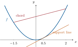
$f$ lies above each support line: for $a$ interior and any $m \in \intcc{f'_g(a)}{f'_d(a)}$ ,

$f(x) \geq f(a) + m(x - a) \qquad (x \in I).$
(Jensen, weighted) For $x_i \in I$ and weights $\lambda_i \geq 0$ , $\sum\lambda_i = 1$ :

$f\Bigl(\sum_i \lambda_i x_i\Bigr) \leq \sum_i \lambda_i f(x_i) .$

Proof. (1) Fix $a$ interior. By Lemma 8.4, the slope $\tau(h) = \frac{f(a + h) - f(a)}{h}$ is an increasing function of $h$ (on both sides, and $\tau(h_-) \leq \tau(h_+)$ for $h_- < 0 < h_+$ ). Hence $\tau$ has a finite limit as $h \to 0^-$ (increasing, bounded above by any right slope) — this is $f'_g(a)$ — and as $h \to 0^+$ ( $f'_d(a)$ ), with $f'_g(a) \leq f'_d(a)$ . Finite one-sided derivatives force continuity at $a$ . Monotonicity in the point: for $a < b$ interior, $f'_d(a) \leq \frac{f(b) - f(a)}{b - a} \leq f'_g(b)$ , again by the slope inequality.

(2) For $x > a$ : $\frac{f(x) - f(a)}{x - a} \geq f'_d(a) \geq m$ ; for $x < a$ : $\frac{f(a) - f(x)}{a - x} \leq f'_g(a) \leq m$ . Both rearrange to the claim.

(3) Induction on the number of points exactly as in the Year 1 volume (the two-point case is the definition) — or in one stroke: apply (2) at $a = \sum\lambda_i x_i$ and average the support-line inequalities at the points $x_i$ with weights $\lambda_i$ : $\sum_i \lambda_i f(x_i) \geq f(a) + m\sum_i\lambda_i(x_i - a) = f(a)$ . ∎

Convexity in one picture: between -1.5 and 2 the graph of f(x) = x2 stays below its chord (the definition) and above the support line at x = 0.5 ( (2)) — every inequality of this chapter’s weekend problem is a rearrangement of these two positions. — Convexity in one picture: between $-1.5$ and $2$ the graph of $f(x) = x^2$ stays below its chord (the definition) and above the support line at $x = 0.5$ (Theorem 8.5 (2)) — every inequality of this chapter’s weekend problem is a rearrangement of these two positions.

Example 8.6 (Endpoint discontinuity)

On $\intcc{0}{1}$ , the function $f(0) = 1$ , $f(x) = 0$ for $x > 0$ is convex but discontinuous at the endpoint $0$ : statement (1) is sharp.

Example 8.7 (Corners and the sheaf of support lines)

For $f(x) = \abs x$ at $a = 0$ : the one-sided derivatives are $f'_g(0) = -1$ and $f'_d(0) = +1$ , and Theorem 8.5 (2) hands out a support line for every slope $m \in \intcc{-1}{1}$ :

\abs x \geq m\,x \qquad (x \in \R,\ -1 \leq m \leq 1),

each an equality exactly on a half-line or at $0$ . A convex function is differentiable at $a$ precisely when the sheaf collapses to a single line ( $f'_g(a) = f'_d(a)$ ); corners carry an interval of tangents. This sheaf is the finite-dimensional germ of the subdifferential of convex optimization — and the reason convex functions are so robust: even where the derivative fails, the supporting geometry survives, which is all that Jensen’s proof used.

Example 8.8 (Power mean inequality)

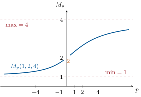
For $0 < p < q$ and positive $x_i$ with weights $\lambda_i$ summing to $1$ , applying Jensen to the convex $t \mapsto t^{q/p}$ at the points $x_i^p$ :

\Bigl(\sum \lambda_i x_i^{p}\Bigr)^{1/p} \leq \Bigl(\sum \lambda_i x_i^{q}\Bigr)^{1/q} :

power means increase with the exponent — containing AM–QM, and, in the limit $p \to 0$ (Exercise 8.6), the AM–GM inequality once more.

The power mean M_p of the values 1, 2, 4 (equal weights), as a function of the exponent p: increasing from = 1 (as p -∈fty) to = 4 (as p +∈fty), through the harmonic (p = -1), geometric (the gap at p = 0, value 2), arithmetic (p = 1) and quadratic (p = 2) means. The whole chain of classical mean inequalities is one increasing curve — proved in this chapter’s weekend problem, Part III. — The power mean $M_p$ of the values $1, 2, 4$ (equal weights), as a function of the exponent $p$ : increasing from $\min = 1$ (as $p \to -\infty$ ) to $\max = 4$ (as $p \to +\infty$ ), through the harmonic ( $p = -1$ ), geometric (the gap at $p = 0$ , value $2$ ), arithmetic ( $p = 1$ ) and quadratic ( $p = 2$ ) means. The whole chain of classical mean inequalities is one increasing curve — proved in this chapter’s weekend problem, Part III.

Example 8.9 (Maximal entropy)

For a probability vector $(p_1, \dots, p_n)$ (positive, summing to $1$ ), the entropy $H(p) = -\sum_i p_i\ln p_i$ satisfies

H(p) \leq \ln n , \qquad\text{with equality iff } p_i = \frac1n \text{ for all } i .

Proof by Jensen (Theorem 8.5 (3)) applied to the concave $\ln$ with weights $p_i$ at the points $\frac{1}{p_i}$ :

H(p) = \sum_i p_i\ln\frac{1}{p_i} \leq \ln\Bigl(\sum_i p_i\,\frac1{p_i}\Bigr) = \ln n ,

equality forcing all points $\frac1{p_i}$ equal (strict concavity), i.e. $p$ uniform. Equivalently, this is Exercise 8.7 with $q$ uniform. Uncertainty is maximized by ignorance uniformly spread — the variational principle behind coding, statistical mechanics, and the entropy appearances of Chapter 22.

Method 8.10 (Finding the convex function behind an inequality)

Most classical inequalities are Jensen in costume; to undress one: (1) normalize so that a weighted average appears (weights positive, summing to $1$ — divide by a total mass if necessary); (2) look at what function is applied inside versus outside the average: the claim “ $f(\text{average}) \leq$ average of $f$ ” names the convex $f$ ; (3) certify convexity by the second derivative, and handle equality via strictness; (4) if no average is visible, take logarithms first — products and powers become averages, and the concavity of $\ln$ carries AM–GM, Young and their relatives (this chapter’s weekend problem runs steps 1–4 on each of them). If even logarithms do not reveal an average, try reading the inequality as monotonicity of slopes (Lemma 8.4) — superadditivity statements like Exercise 8.9 live there.

Remark 8.11 (Common pitfalls)

(i) Convexity is not preserved by products: $x$ and $(x - 1)^2$ are convex on $\intcc{0}{2}$ , but their product $x(x-1)^2$ has second derivative $6x - 4$ , negative on $\intco{0}{\frac23}$ — not convex; nor is convexity preserved by composition without monotonicity (Exercise 8.10). (ii) Jensen flips for concave functions: half the classical inequalities are the concave $\ln$ -version; applying the convex form to $\ln$ is the quickest way to prove AM–GM backwards. (iii) Midpoint convexity alone does not imply convexity — continuity (or mere boundedness) is needed (Exercise 8.8); the pathological counterexamples live beyond this book’s axioms. (iv) A convex function on an open interval is continuous, even locally Lipschitz (Exercise 8.12); at endpoints, nothing is free. (v) Derivatives obey Darboux but need not be continuous (Example 8.15): “ $f'$ has no jumps” never means “ $f'$ is continuous”.

8.3 The Darboux property

Theorem 8.12 (Darboux)

Let $f$ be differentiable on an interval $I$ . Then $f'$ takes every value between any two of its values — even though $f'$ need not be continuous.

Proof. Let $a < b$ in $I$ and $v$ strictly between $f'(a)$ and $f'(b)$ , say $f'(a) < v < f'(b)$ . The function $g(x) = f(x) - vx$ is differentiable with $g'(a) < 0 < g'(b)$ : its minimum on $\intcc{a}{b}$ (attained: continuity on a compact) is not at $a$ (just after $a$ , $g$ decreases below $g(a)$ ) nor at $b$ (just before $b$ , $g$ is below $g(b)$ ): it is interior, and there $g'(c) = 0$ , i.e. $f'(c) = v$ . (This was a Year 1 starred exercise; its place in the theory is here.) ∎

Example 8.13 (Which functions are derivatives?)

Darboux’s theorem is a non-existence machine. The floor function $\lfloor x\rfloor$ is not the derivative of any function on $\R$ : it takes the values $0$ and $1$ but skips $\frac12$ on $\intcc{0}{1}$ , which Theorem 8.12 forbids for derivatives. The same verdict hits every function with a jump — sign, Heaviside, all step functions — however innocent they look; their “antiderivatives” ( $\abs x$ for sign, etc.) exist only away from the jump and knot there with a corner. Contrast: the wildly discontinuous $f'$ of Example 8.15 is a derivative — its discontinuity is an oscillation, which Darboux tolerates. The boundary between the two behaviours is exactly the no-jumps corollary below.

Corollary 8.14

A derivative has no jump discontinuities: if $f'(a^-)$ and $f'(a^+)$ exist, they equal $f'(a)$ . The discontinuities of a derivative are always of oscillation type ( $x^2\sin\frac1x$ ’s derivative at $0$ , Year 1 volume).

Proof. If $f'(a^+) = \lim_{x\to a^+} f'(x)$ exists and differs from $f'(a)$ , values strictly between them would be skipped by $f'$ on a right neighborhood — contradicting Darboux on intervals $\intcc{a}{a + h}$ . (Alternatively: the mean value theorem forces $f'(a) = \lim_{h\to0^+} \frac{f(a+h)-f(a)}{h} = f'(a^+)$ , the difference quotient being an $f'$ -value at an intermediate point.) Same on the left. ∎

Example 8.15 (The canonical oscillating derivative)

Let $f(x) = x^2\sin\frac1x$ for $x \neq 0$ and $f(0) = 0$ . At $0$ : $\bigl|\frac{f(h) - f(0)}{h}\bigr| = \abs{h\sin\frac1h} \leq \abs h \to 0$ , so $f'(0) = 0$ exists. Away from $0$ ,

f'(x) = 2x\sin\frac1x - \cos\frac1x ,

whose first term tends to $0$ while $\cos\frac1x$ oscillates through $\intcc{-1}{1}$ on every interval $\intoo{0}{\delta}$ : the limit $f'(0^+)$ does not exist. So $f'$ is defined everywhere but discontinuous at $0$ — and, exactly as Corollary 8.14 predicts, the discontinuity is an oscillation, not a jump: on each $\intoo{0}{\delta}$ , $f'$ still sweeps a full interval around $0$ . Derivatives can be wild, but only in the Darboux-compatible way.

Remark 8.16 (Where this chapter is used)

Convexity is the engine of the inequality industry: this chapter’s weekend problem manufactures Young, Hölder, Minkowski and the power-mean chain from it, which Chapter 5’s norm theory and Chapter 9’s integral estimates consume; Jensen reappears in probability as the moment inequalities of Chapter 22. Monotone regularity returns in Chapter 9 (monotone functions are integrable) and, in the Year 3 volume, as the almost-everywhere differentiability of monotone functions — where “countably many jumps” becomes the first step of Lebesgue’s theory.

8.4 Exercises

Exercise 8.1 ★

Determine the discontinuity sets and the jump sizes: $\lfloor x \rfloor$ ; $\;x - \lfloor x\rfloor$ ; $\;\lfloor x \rfloor + \sqrt{x - \lfloor x\rfloor}$ ; the function of the example following Theorem 8.1 restricted to dyadic rationals $r_n$ .

Solution

Solution of Exercise 8.1.

$\lfloor x\rfloor$ : jumps of size $1$ at every integer. $x - \lfloor x\rfloor$ : jumps of size $-1$ at integers (left limit $1$ , value $0$ ). $\lfloor x\rfloor + \sqrt{x - \lfloor x\rfloor}$ : at an integer $n$ , left limit $(n - 1) + 1 = n$ and value $n$ : continuous everywhere (the square root repairs the jump), though not differentiable at integers. The rational-jump function: restricting the construction to an enumeration of the dyadics, it jumps by $2^{-n}$ exactly at the $n$ -th dyadic rational and is continuous elsewhere.

Exercise 8.2 ★

Prove that an increasing function $f \colon I \to \R$ with the intermediate value property (its image of any subinterval is an interval) is continuous.

Solution

Solution of Exercise 8.2.

Suppose $f$ increasing has a discontinuity at an interior $a$ : then $f(a^-) < f(a^+)$ (Theorem 8.1) and the image of $I$ misses the nonempty open interval $\intoo{f(a^-)}{f(a^+)}$ except possibly the single value $f(a)$ : the image of any subinterval containing $a$ in its interior is not an interval (it has a gap on at least one side of $f(a)$ ). This contradicts the intermediate value property. Endpoint discontinuities are excluded the same way with one-sided gaps.

Exercise 8.3 ★

Which of the following are convex on their domain? $x \mapsto x\ln x$ ( $x > 0$ ); $\;x \mapsto \ln(1 + \eu^x)$ ; $\;x \mapsto \sqrt{1 + x^2}$ ; $\;x \mapsto x^3$ .

Solution

Solution of Exercise 8.3.

$x\ln x$ : second derivative $\frac1x > 0$ : convex. $\ln(1 + \eu^x)$ : derivative $\frac{\eu^x}{1 + \eu^x} = 1 - \frac{1}{1 + \eu^x}$ , increasing: convex. $\sqrt{1 + x^2}$ : second derivative $(1 + x^2)^{-3/2} > 0$ : convex. $x^3$ : not convex on $\R$ ( $f'' = 6x$ changes sign); convex only on $\R_+$ .

Exercise 8.4 ★★

Let $f$ be convex on $\R$ and bounded above. Prove that $f$ is constant. (If $f(a) \neq f(b)$ , the slope inequality propagates the nonzero chord slope: beyond the point with the larger value, $f$ grows at least linearly — contradicting boundedness. Treat both signs of the slope.) Deduce that a convex function on $\R$ with an asymptote at both ends is affine.

Solution

Solution of Exercise 8.4.

Suppose $f(a) \neq f(b)$ , say $f(b) > f(a)$ with $a < b$ (the case $f(b) < f(a)$ is symmetric, looking left). For $x > b$ , the slope inequality (Lemma 8.4) on $a < b < x$ gives

\frac{f(x) - f(a)}{x - a} \geq \frac{f(b) - f(a)}{b - a} = m > 0 \quad\Longrightarrow\quad f(x) \geq f(a) + m(x - a) \xrightarrow[x\to+\infty]{} +\infty,

contradicting boundedness above. Hence $f$ is constant.

Asymptotes: if $f(x) - (\alpha x + \beta) \to 0$ at $+\infty$ and $f(x) - (\alpha' x + \beta') \to 0$ at $-\infty$ , the convex function $g(x) = f(x) - (\alpha x + \beta)$ is bounded above near $+\infty$ ; convexity plus an asymptote at $-\infty$ (which forces $\alpha' \leq \alpha$ then $\alpha' = \alpha$ by comparing slopes at $\mp\infty$ : slopes of a convex function increase) makes $g$ bounded above on all of $\R$ , hence constant $= 0$ in the limit: $f$ is affine.

Exercise 8.5 ★★

Let $f$ be differentiable on $I$ with $f'$ monotone. Prove that $f'$ is continuous (combine Theorem 8.1 and Corollary 8.14).

Solution

Solution of Exercise 8.5.

$f'$ is monotone, so by Theorem 8.1 its only possible discontinuities are jumps, with one-sided limits existing everywhere. By Corollary 8.14, a derivative has no jump discontinuities. Hence $f'$ has no discontinuities at all: continuous.

Exercise 8.6 ★★

(Geometric mean as a limit) For positive $x_i$ and weights $\lambda_i$ summing to $1$ , prove

\lim_{p \to 0^+} \Bigl(\sum_i \lambda_i x_i^p\Bigr)^{1/p} = \prod_i x_i^{\lambda_i} ,

via $x_i^p = \eu^{p\ln x_i} = 1 + p\ln x_i + O(p^2)$ , and deduce the weighted AM–GM inequality from Example 8.8.

Solution

Solution of Exercise 8.6.

Take logarithms:

\frac1p \ln\Bigl(\sum_i \lambda_i x_i^p\Bigr) = \frac1p \ln\Bigl(1 + p\sum_i \lambda_i \ln x_i + O(p^2)\Bigr) = \sum_i \lambda_i \ln x_i + O(p) \xrightarrow[p \to 0^+]{} \sum_i \lambda_i \ln x_i ,

using $\sum\lambda_i = 1$ and $\ln(1 + u) = u + O(u^2)$ . Exponentiating gives the geometric mean. Now for every $p \in \intoo{0}{1}$ , the power-mean inequality (Example 8.8, exponents $p < 1$ ) gives

\Bigl(\sum_i \lambda_i x_i^p\Bigr)^{1/p} \leq \sum_i\lambda_i x_i ;

letting $p \to 0^+$ on the left yields $\prod_i x_i^{\lambda_i} \leq \sum_i \lambda_i x_i$ : the weighted AM–GM inequality.

Exercise 8.7 ★★

(Entropy inequality) Using strict convexity of $t \mapsto t\ln t$ , prove that for positive $p_i, q_i$ with $\sum p_i = \sum q_i = 1$ :

\sum_i p_i \ln\frac{p_i}{q_i} \geq 0 ,

with equality iff $p = q$ . (Write the left side as $\sum q_i\, \varphi\bigl(\frac{p_i}{q_i}\bigr)$ with $\varphi(t) = t\ln t$ and apply Jensen with weights $q_i$ .)

Solution

Solution of Exercise 8.7.

With $\varphi(t) = t\ln t$ (convex: $\varphi'' = \frac1t > 0$ ) and weights $q_i$ at the points $t_i = \frac{p_i}{q_i}$ :

\sum_i p_i \ln\frac{p_i}{q_i} = \sum_i q_i\, \varphi\Bigl(\frac{p_i}{q_i}\Bigr) \;\geq\; \varphi\Bigl(\sum_i q_i \frac{p_i}{q_i}\Bigr) = \varphi(1) = 0 ,

by Jensen (Theorem 8.5 (3)). Equality in Jensen for a strictly convex function forces all the points $t_i$ to coincide: $\frac{p_i}{q_i}$ constant, and summing, the constant is $1$ : $p = q$ . (This quantity — the Kullback–Leibler divergence — returns in Chapter 22’s world.)

Exercise 8.8 ★★★

(Midpoint convexity) $f \colon I \to \R$ is midpoint convex when $f\bigl(\frac{x+y}{2}\bigr) \leq \frac{f(x) + f(y)}{2}$ always. Prove that a continuous midpoint convex function is convex. (Establish the convexity inequality for dyadic weights $\frac{k}{2^m}$ by induction on $m$ , then pass to the limit using density and continuity.)

Solution

Solution of Exercise 8.8.

Dyadic weights. By induction on $m$ : the case $m = 1$ is the hypothesis. For weight $\lambda = \frac{k}{2^{m+1}}$ (odd $k$ ), write $\lambda = \frac12(\lambda_1 + \lambda_2)$ with $\lambda_j = \frac{k \mp 1}{2^{m+1}}$ , both of denominator $2^m$ after simplification; then

f\bigl(\lambda x + (1{-}\lambda)y\bigr) = f\Bigl(\tfrac{u + v}{2}\Bigr) \leq \frac{f(u) + f(v)}{2} \leq \lambda f(x) + (1 - \lambda) f(y),

where $u = \lambda_1 x + (1 - \lambda_1)y$ and $v = \lambda_2 x + (1-\lambda_2)y$ , using midpoint convexity then the induction hypothesis on $u, v$ .

Passage to the limit. For arbitrary $\lambda \in \intcc{0}{1}$ , take dyadics $\lambda_n \to \lambda$ : continuity of $f$ and of the affine maps passes the inequality $f(\lambda_n x + (1-\lambda_n)y) \leq \lambda_n f(x) + (1-\lambda_n)f(y)$ to the limit: $f$ is convex.

Exercise 8.9 ★★★

Let $f$ be convex on $\intco{0}{+\infty}$ with $f(0) \leq 0$ . Prove that $x \mapsto \frac{f(x)}{x}$ is increasing on $\intoo{0}{+\infty}$ , and deduce that for convex $f$ with $f(0) = 0$ : $f(x + y) \geq f(x) + f(y)$ for $x, y \geq 0$ (superadditivity).

Solution

Solution of Exercise 8.9.

For $0 < x < y$ : the slope inequality (Lemma 8.4) at the points $0 < x < y$ gives

\frac{f(x) - f(0)}{x} \leq \frac{f(y) - f(0)}{y}, \qquad\text{i.e.}\qquad \frac{f(x)}{x} \leq \frac{f(y)}{y} + f(0)\Bigl(\frac1x - \frac1y\Bigr).

Since $f(0) \leq 0$ and $\frac1x - \frac1y > 0$ , the last term is $\leq 0$ : $\frac{f(x)}{x} \leq \frac{f(y)}{y}$ . So $x \mapsto \frac{f(x)}x$ increases.

Superadditivity for $f(0) = 0$ : for $x, y > 0$ (the cases with a zero variable are trivial),

f(x) = x\,\frac{f(x)}{x} \leq x\,\frac{f(x+y)}{x+y}, \qquad f(y) \leq y\,\frac{f(x+y)}{x+y},

by the monotonicity just proved; adding gives $f(x) + f(y) \leq f(x+y)$ .

Exercise 8.10 ★

Let $f$ be convex on $I$ and $g$ convex increasing on an interval containing $f(I)$ . Prove that $g \circ f$ is convex, and show by a counterexample that monotonicity of $g$ cannot be dropped.

Solution

Solution of Exercise 8.10.

For $x, y \in I$ and $\lambda \in \intcc01$ : convexity of $f$ , then monotonicity of $g$ , then convexity of $g$ :

g\bigl(f(\lambda x + (1{-}\lambda)y)\bigr) \leq g\bigl(\lambda f(x) + (1{-}\lambda)f(y)\bigr) \leq \lambda\,g(f(x)) + (1{-}\lambda)\,g(f(y)).

Counterexample without monotonicity: $g(t) = -t$ is convex (affine) but decreasing, $f(x) = x^2$ is convex, and $g \circ f = -x^2$ is strictly concave.

Exercise 8.11 ★★

(Hermite–Hadamard) Let $f$ be convex and continuous on $\intcc{a}{b}$ . Prove

f\Bigl(\frac{a+b}{2}\Bigr) \;\leq\; \frac{1}{b - a}\int_a^b f(t)\,\dd t \;\leq\; \frac{f(a) + f(b)}{2} .

(Left: integrate a support line at the midpoint. Right: bound $f$ by the chord.)

Solution

Solution of Exercise 8.11.

Left inequality: let $m = \frac{a+b}2$ and take a support line at $m$ (Theorem 8.5 (2)): $f(t) \geq f(m) + \mu(t - m)$ for all $t \in \intcc ab$ . Integrating over $\intcc{a}{b}$ : the linear term integrates to $\mu\int_a^b(t - m)\dd t = 0$ (symmetry around $m$ ), so $\int_a^b f \geq (b - a)f(m)$ .

Right inequality: on $\intcc ab$ , convexity bounds $f$ by its chord: $f(t) \leq f(a) + \frac{f(b) - f(a)}{b - a}(t - a)$ . Integrating: $\int_a^b f \leq (b-a)f(a) + \frac{f(b) - f(a)}{b - a}\cdot\frac{(b-a)^2}2 = (b - a)\,\frac{f(a) + f(b)}2$ . Divide by $b - a$ .

Exercise 8.12 ★★★

Prove that a convex function on an open interval $I$ is locally Lipschitz: for every segment $\intcc{a}{b} \subseteq I$ and margin $\delta > 0$ with $\intcc{a - \delta}{b + \delta} \subseteq I$ , the restriction of $f$ to $\intcc{a}{b}$ is Lipschitz, with constant $\max\Bigl(\bigl|\frac{f(a) - f(a - \delta)}{\delta}\bigr|, \bigl|\frac{f(b + \delta) - f(b)}{\delta}\bigr|\Bigr)$ (trap every chord slope between these two by the slope inequality).

Solution

Solution of Exercise 8.12.

Let $a - \delta < a \leq x < y \leq b < b + \delta$ , all in $I$ . Two applications of the slope inequality (Lemma 8.4), first to $a - \delta < a \leq x < y$ , then to $x < y \leq b < b + \delta$ :

\frac{f(a) - f(a - \delta)}{\delta} \leq \frac{f(y) - f(x)}{y - x} \leq \frac{f(b + \delta) - f(b)}{\delta}

(chord slopes increase when both endpoints move right). Hence every chord slope inside $\intcc ab$ is trapped between two fixed numbers, and

\abs{f(y) - f(x)} \leq K\,\abs{y - x}, \qquad K = \max\Bigl(\Bigl|\frac{f(a) - f(a-\delta)}{\delta}\Bigr|, \Bigl|\frac{f(b+\delta) - f(b)}{\delta}\Bigr|\Bigr):

$f$ is Lipschitz on $\intcc ab$ . Every point of the open $I$ has such a segment-with-margin around it: locally Lipschitz, hence (again) continuous on $I$ .

8.5 Problem: The Convexity Toolbox

One definition — the chord above the graph — generates the entire toolbox of classical inequalities. This weekend problem builds it in logical order: convexity criteria and strict Jensen, then Young, Hölder and Minkowski (the birth certificates of the $p$ -norms), the complete power-mean chain from the minimum to the maximum, and two crown dividends — Carleman’s inequality, and Hölder read as a duality. Everything is proved; nothing is imported.

Problem 8.1

Weekend problem — Young, Hölder, Minkowski, and the power-mean chain

Throughout, $p, q > 1$ are conjugate exponents: $\frac1p + \frac1q = 1$ ; vectors are $a = (a_1, \dots, a_n) \in \R^n$ ; weights $\lambda_i > 0$ satisfy $\sum_i\lambda_i = 1$ .

Part I — Criteria and strict Jensen.

Let $f$ be differentiable on an interval $I$ . Prove that $f$ is convex if and only if $f'$ is increasing (one direction by passing to the limit in the slope inequality Lemma 8.4; the other by the mean value theorem). Deduce the $C^2$ criterion $f'' \geq 0$ .
Suppose $f''> 0$ on $I$ . Prove that $f$ is strictly convex (strict inequality for $x \neq y$ and $\lambda \in \intoo01$ ), and that a strictly convex function satisfies Jensen’s inequality (Theorem 8.5 (3)) with equality only when all the $x_i$ coincide.
Certify the toolbox’s raw materials: $-\ln$ is strictly convex on $\intoo{0}{+\infty}$ ; $t \mapsto t^r$ is strictly convex there for $r > 1$ and strictly concave for $0 < r < 1$ ; $\exp$ is strictly convex on $\R$ .
(Young’s inequality) For $a, b \geq 0$ , prove

$ab \;\leq\; \frac{a^p}{p} + \frac{b^q}{q},$

with equality if and only if $a^p = b^q$ (apply the concavity of $\ln$ to the two points $a^p, b^q$ with weights $\frac1p, \frac1q$ ).
Re-derive weighted AM–GM in one line from the concavity of $\ln$ :

$\prod_i x_i^{\lambda_i} \leq \sum_i\lambda_ix_i \qquad (x_i > 0),$

with the equality case; compare with the limit route of Exercise 8.6.

Part II — Hölder and Minkowski. Write $\norm{a}_p = \bigl(\sum_i \abs{a_i}^p\bigr)^{1/p}$ and $\norm{a}_\infty = \max_i\abs{a_i}$ .

(Hölder) Prove

$\sum_{i=1}^{n}\abs{a_ib_i} \;\leq\; \norm a_p\,\norm b_q ,$

with equality iff the vectors $(\abs{a_i}^p)$ and $(\abs{b_i}^q)$ are proportional (normalize $\norm a_p = \norm b_q = 1$ and apply Young termwise).
Identify the special cases: $p = q = 2$ (Cauchy–Schwarz), and the endpoint pair $(p, q) = (1, \infty)$ : state and prove $\sum\abs{a_ib_i} \leq \norm a_1\norm b_\infty$ .
(Minkowski) For $p \geq 1$ , prove

$\norm{a + b}_p \leq \norm a_p + \norm b_p$

(write $\abs{a_i + b_i}^p \leq \abs{a_i + b_i}^{p-1}(\abs{a_i} + \abs{b_i})$ and apply Hölder to each product). Conclude: $\norm\cdot_p$ is a norm on $\R^n$ for every $p \in \intco{1}{+\infty}$ , completing the picture of Chapter 5.
Integral versions: for $f, g$ continuous on $\intcc{a}{b}$ , state and prove Hölder and Minkowski for $\norm f_p = \bigl(\int_a^b\abs f^p\bigr)^{1/p}$ (same proofs, with the strict positivity of the integral for the equality discussion).
Prove the monotonicity $\norm a_q \leq \norm a_p$ for $1 \leq p \leq q$ , the limit $\norm a_p \to \norm a_\infty$ as $p \to \infty$ , and the reverse comparison with the sharp constant:

$\norm a_p \leq n^{\frac1p - \frac1q}\,\norm a_q$

(Hölder against the constant vector). Identify the vectors achieving each equality.
(Interpolation) For $1 \leq p < r < q$ and $\theta \in \intoo01$ with $\frac1r = \frac\theta p + \frac{1-\theta}q$ , prove

$\norm a_r \leq \norm a_p^{\theta}\, \norm a_q^{1-\theta}$

(apply Hölder with exponents $\frac{p}{\theta r}$ and $\frac{q}{(1-\theta)r}$ to $\abs{a_i}^{\theta r}\abs{a_i}^{(1-\theta)r}$ ).

Part III — The power-mean chain, complete. For $p \neq 0$ set $M_p = \bigl(\sum_i\lambda_i x_i^p\bigr)^{1/p}$ ( $x_i > 0$ ), and $M_0 = \prod_i x_i^{\lambda_i}$ .

Prove that $p \mapsto M_p$ is increasing on all of $\R^*$ : treat $p < q < 0$ by the reciprocal identity $M_{-p}(x) = M_p(1/x)^{-1}$ , and bridge through $0$ by showing $M_p \leq M_0 \leq M_q$ for $p < 0 < q$ (apply the concavity of $\ln$ to $x_i^q$ , and the reversed inequality for negative exponents).
Prove the limits $M_p \to \max_i x_i$ as $p \to +\infty$ and $M_p \to \min_i x_i$ as $p \to -\infty$ .
Write out the chain $\min \leq \mathrm{HM} \leq \mathrm{GM} \leq \mathrm{AM} \leq \mathrm{QM} \leq \max$ for equal weights, and prove the classic consequence: for positive $a_1, \dots, a_n$ ,

$\Bigl(\sum_i a_i\Bigr)\Bigl(\sum_i\frac1{a_i}\Bigr) \geq n^2 .$
Relate means to norms: for equal weights $\lambda_i = \frac1n$ , $M_p(x) = n^{-1/p}\norm x_p$ . Reconcile the two monotonicities — means increase with $p$ while norms decrease (question 10) — in one sentence about the factor $n^{-1/p}$ .
Determine the equality cases along the whole chain of question 14 (positive weights): equality anywhere forces all $x_i$ equal — strict convexity pays off.

Part IV — Dividends.

(Young with a knob) For $a, b \geq 0$ and $\varepsilon > 0$ , prove

$ab \leq \varepsilon\,\frac{a^p}{p} + \varepsilon^{-q/p}\,\frac{b^q}{q},$

and the workhorse case $ab \leq \varepsilon a^2 + \frac{b^2}{4\varepsilon}$ : the absorption trick used throughout analysis.
(Toward Carleman) Let $c_k = \frac{(k+1)^k}{k^{k-1}}$ . Prove the telescoping identity $\prod_{k=1}^{n}c_k = (n+1)^n$ , and deduce, by AM–GM applied to the numbers $c_ka_k$ ,

$(a_1a_2\cdots a_n)^{1/n} \leq \frac{1}{n(n+1)}\sum_{k=1}^{n} c_k a_k \qquad (a_k > 0).$
(Carleman’s inequality) Sum over $n$ , exchange the order of summation (positive summable families, Theorem 7.14), and use $\sum_{n \geq k}\frac{1}{n(n+1)} = \frac1k$ and $c_k/k = \bigl(1 + \frac1k\bigr)^k < \eu$ to conclude: for every convergent $\sum a_k$ with positive terms,

$\sum_{n=1}^{\infty}(a_1a_2\cdots a_n)^{1/n} \;\leq\; \eu\sum_{k=1}^{\infty}a_k .$
For $f$ continuous and positive on $\intcc{0}{1}$ , prove

$\Bigl(\int_0^1 f\Bigr)\Bigl(\int_0^1\frac1f\Bigr) \geq 1,$

with equality iff $f$ is constant (Cauchy–Schwarz on $\sqrt f\cdot\frac1{\sqrt f}$ ).
(Geometry of the balls) Using the equality case of Minkowski, show that for $1 < p < \infty$ the unit sphere of $\norm\cdot_p$ contains no segment (the norm is strictly convex in the sense of Problem 5.1), whereas for $p = 1$ and $p = \infty$ it does: exhibit the flat pieces.

Part V — Duality and synthesis.

(Hölder as duality) Prove that for every $a \in \R^n$ ,

$\norm a_p = \max_{\norm b_q \leq 1}\ \sum_i a_ib_i ,$

exhibiting a maximizing $b$ explicitly. (The $p$ -norm is the dual of the $q$ -norm — the finite-dimensional germ of $L^p$ duality.)
(Moments) Let $X$ be a random variable taking finitely many positive values $x_i$ with probabilities $\lambda_i$ . Restate question 12 as: $r \mapsto \E[X^r]^{1/r}$ is increasing — the moment (Lyapunov) inequality, to be reused in Chapter 22.
Solve with named tools, in two lines each: (i) for positive $a, b, c$ : $a^3 + b^3 + c^3 \geq \frac{(a+b+c)^3}{9}$ ; (ii) for positive $x_1, \dots, x_n$ : $\bigl(\sum_i\sqrt{x_i}\bigr)^2 \leq n\sum_i x_i$ .
(Synthesis) Draw the genealogy in five sentences: chord definition to slope lemma; slopes to support lines to Jensen; $\ln$ ’s concavity to Young to Hölder to Minkowski to the $p$ -norms; Jensen to the power-mean chain to moments; AM–GM to Carleman. Name the summits (Hölder–Minkowski; Carleman), and state where the toolbox is headed: the $L^p$ spaces of the Year 3 volume, whose axioms are exactly questions 6 and 8.

Solution

Solution of Problem 8.1.

1. Convex $\Rightarrow$ $f'$ increasing: for $a < b$ , the slope inequality gives, for small $h > 0$ , $\frac{f(a+h) - f(a)}h \leq \frac{f(b) - f(a)}{b-a} \leq \frac{f(b) - f(b-h)}{h}$ ; letting $h \to 0$ : $f'(a) \leq \frac{f(b) - f(a)}{b - a} \leq f'(b)$ . Conversely, if $f'$ increases and $x < y < z$ : the mean value theorem gives $c_1 \in \intoo{x}{y}$ , $c_2 \in \intoo yz$ with

\frac{f(y) - f(x)}{y - x} = f'(c_1) \leq f'(c_2) = \frac{f(z) - f(y)}{z - y},

and this three-point slope inequality, applied with $y = \lambda x + (1 - \lambda)z$ , rearranges into the convexity inequality. For $C^2$ : $f'' \geq 0$ iff $f'$ increases.

2. If $f'' > 0$ , $f'$ is strictly increasing, and the mean value computation above gives a strict inequality between the two chord slopes: strict convexity. Strict support: at an interior $a$ with support slope $m$ , if $f(x_0) = f(a) + m(x_0 - a)$ for some $x_0 \neq a$ , then on the segment from $a$ to $x_0$ the support line and the chord coincide, and strict convexity at the midpoint gives $f\bigl(\frac{a + x_0}2\bigr) < f(a) + m\,\frac{x_0 - a}2$ , contradicting the support inequality. So $f(x) > f(a) + m(x - a)$ for all $x \neq a$ . Strict Jensen: with $a = \sum\lambda_ix_i$ , averaging the support inequalities gives $\sum\lambda_if(x_i) \geq f(a)$ , with equality iff each term is an equality, i.e. iff every $x_i = a$ .

3. $(-\ln)'' = \frac1{t^2} > 0$ ; $(t^r)'' = r(r - 1)t^{r-2}$ , positive for $r > 1$ , negative for $0 < r < 1$ ; $\exp'' = \exp > 0$ . All strict by question 2.

4. The cases $ab = 0$ are trivial. For $a, b > 0$ , concavity of $\ln$ at the points $a^p, b^q$ with weights $\frac1p, \frac1q$ :

\ln\Bigl(\frac{a^p}p + \frac{b^q}q\Bigr) \geq \frac1p\ln(a^p) + \frac1q\ln(b^q) = \ln(ab),

and $\ln$ increases: $ab \leq \frac{a^p}p + \frac{b^q}q$ . Equality iff the two points coincide (strict concavity): $a^p = b^q$ .

5. Concavity of $\ln$ with weights $\lambda_i$ : $\ln\bigl(\sum\lambda_ix_i\bigr) \geq \sum\lambda_i\ln x_i = \ln\prod x_i^{\lambda_i}$ ; exponentiate. Equality iff all $x_i$ equal (question 2). The route of Exercise 8.6 obtained the same inequality as a limit of power means; here it is one application of Jensen — the toolbox has redundancy built in.

6. If $a = 0$ or $b = 0$ the inequality is trivial. Normalize: replacing $a$ by $a/\norm a_p$ and $b$ by $b/\norm b_q$ , we may assume $\norm a_p = \norm b_q = 1$ and must show $\sum\abs{a_ib_i} \leq 1$ . Young termwise:

\sum_i\abs{a_i}\abs{b_i} \leq \sum_i\Bigl(\frac{\abs{a_i}^p}{p} + \frac{\abs{b_i}^q}{q}\Bigr) = \frac1p + \frac1q = 1 .

Equality iff each Young inequality is tight: $\abs{a_i}^p = \abs{b_i}^q$ for all $i$ — after undoing the normalization, $(\abs{a_i}^p)$ proportional to $(\abs{b_i}^q)$ .

7. $p = q = 2$ is Cauchy–Schwarz with the same equality case (proportionality). Endpoint: $\sum\abs{a_ib_i} \leq \bigl(\max_i\abs{b_i}\bigr)\sum_i\abs{a_i} = \norm a_1\norm b_\infty$ , immediate termwise.

8. For $p = 1$ it is the triangle inequality termwise. For $p > 1$ , with $q$ conjugate:

\norm{a+b}_p^p = \sum_i\abs{a_i + b_i}^p \leq \sum_i\abs{a_i+b_i}^{p-1}\abs{a_i} + \sum_i\abs{a_i+b_i}^{p-1}\abs{b_i},

and Hölder on each sum, noting $(p - 1)q = p$ :

\sum_i\abs{a_i+b_i}^{p-1}\abs{a_i} \leq \Bigl(\sum_i\abs{a_i+b_i}^{p}\Bigr)^{1/q}\norm a_p = \norm{a + b}_p^{p/q}\,\norm a_p ,

likewise with $b$ . Hence $\norm{a+b}_p^p \leq \norm{a + b}_p^{p/q}\bigl(\norm a_p + \norm b_p\bigr)$ ; if $a + b \neq 0$ , divide by $\norm{a+b}_p^{p/q}$ and use $p - \frac pq = 1$ . With homogeneity and separation (clear), $\norm\cdot_p$ is a norm on $\R^n$ .

9. For continuous $f, g$ on $\intcc ab$ : Hölder

\int_a^b\abs{fg} \leq \Bigl(\int_a^b\abs f^p\Bigr)^{1/p}\Bigl(\int_a^b\abs g^q\Bigr)^{1/q}

by the same normalization plus pointwise Young, integrated; and Minkowski $\norm{f + g}_p \leq \norm f_p + \norm g_p$ by the same splitting, Hölder on each piece. Separation of the norm uses strict positivity: a continuous $\abs f^p$ with zero integral vanishes identically (Year 1 volume).

10. Monotonicity: we may assume $\norm a_p = 1$ ; then each $\abs{a_i} \leq 1$ , so $\abs{a_i}^q \leq \abs{a_i}^p$ and $\norm a_q^q \leq 1$ : $\norm a_q \leq 1 = \norm a_p$ . Equality requires $\abs{a_i}^q = \abs{a_i}^p$ for every $i$ , i.e. each $\abs{a_i} \in \{0, 1\}$ ; with $\sum\abs{a_i}^p = 1$ this leaves exactly one coordinate of modulus $1$ : equality iff $a$ has at most one nonzero coordinate. Limit: $\norm a_\infty \leq \norm a_p \leq n^{1/p}\norm a_\infty$ , and $n^{1/p} \to 1$ . Reverse comparison: Hölder with exponents $\frac qp$ and its conjugate $\frac{q}{q-p}$ , applied to $\abs{a_i}^p\cdot 1$ :

\norm a_p^p = \sum_i\abs{a_i}^p\cdot 1 \leq \Bigl(\sum_i\abs{a_i}^{q}\Bigr)^{p/q}\,n^{1 - p/q} = \norm a_q^{p}\; n^{1-p/q},

whence $\norm a_p \leq n^{\frac1p - \frac1q}\norm a_q$ , with equality iff all $\abs{a_i}$ are equal (the Hölder equality case against the constant vector).

11. Write $\abs{a_i}^r = \abs{a_i}^{\theta r}\,\abs{a_i}^{(1-\theta)r}$ and apply Hölder with the conjugate exponents $\frac{p}{\theta r}$ and $\frac{q}{(1-\theta)r}$ (conjugate precisely because $\frac{\theta r}p + \frac{(1-\theta)r}q = 1$ ):

\norm a_r^r = \sum_i \abs{a_i}^{\theta r}\abs{a_i}^{(1-\theta)r} \leq \Bigl(\sum_i\abs{a_i}^{p}\Bigr)^{\theta r/p} \Bigl(\sum_i\abs{a_i}^{q}\Bigr)^{(1-\theta)r/q} = \norm a_p^{\theta r}\,\norm a_q^{(1-\theta)r} .

Take $r$ -th roots: the $p$ -norms are log-convex in $\frac1p$ .

12. Both negative: if $p < q < 0$ then $0 < -q < -p$ , and $M_{-q}(y) \leq M_{-p}(y)$ for the positive exponents (course case, Example 8.8) applied to $y = (1/x_i)$ ; inverting the identity $M_p(x) = M_{-p}(1/x)^{-1}$ reverses the inequality into $M_p(x) \leq M_q(x)$ . Bridge: for $q > 0$ , concavity of $\ln$ gives $\ln M_q = \frac1q\ln\bigl(\sum\lambda_ix_i^q\bigr) \geq \frac1q\sum\lambda_i\ln x_i^q = \ln M_0$ ; for $p < 0$ , the same concavity gives $\ln\bigl(\sum\lambda_ix_i^p\bigr) \geq p\sum\lambda_i\ln x_i$ , and dividing by $p < 0$ flips: $\ln M_p \leq \ln M_0$ . Hence $M_p \leq M_0 \leq M_q$ whenever $p < 0 < q$ : with the two same-sign cases, $M$ increases on all of $\R^*$ (and through $0$ ).

13. Let $x_{\max} = \max x_i$ , attained at $i^*$ . For $p > 0$ :

\lambda_{i^*}^{1/p}\,x_{\max} \leq M_p \leq x_{\max},

and $\lambda_{i^*}^{1/p} \to 1$ : $M_p \to x_{\max}$ . For $p \to -\infty$ : $M_p(x) = M_{-p}(1/x)^{-1} \to \bigl(\max_i\frac1{x_i}\bigr)^{-1} = \min_ix_i$ .

14. With $\lambda_i = \frac1n$ , the chain $M_{-\infty} \leq M_{-1} \leq M_0 \leq M_1 \leq M_2 \leq M_{+\infty}$ reads

\min \leq \frac{n}{\sum\frac1{a_i}} \leq \Bigl(\prod a_i\Bigr)^{1/n} \leq \frac{\sum a_i}{n} \leq \sqrt{\frac{\sum a_i^2}{n}} \leq \max .

AM–HM ( $M_{-1} \leq M_1$ ) rearranges directly into $\bigl(\sum a_i\bigr)\bigl(\sum\frac1{a_i}\bigr) \geq n^2$ .

15. With equal weights, $M_p(x) = \bigl(\frac1n\sum\abs{x_i}^p\bigr)^{1/p} = n^{-1/p}\norm x_p$ . As $p$ grows, $\norm x_p$ decreases (question 10) but the normalizer $n^{-1/p}$ increases faster, and the product increases (question 12): means average, norms accumulate, and the factor $n^{-1/p}$ is exactly the exchange rate between the two bookkeeping conventions.

16. Each link is an instance of strict Jensen (question 2) with the strictly convex/concave functions of question 3 ( $t^{q/p}$ , $\ln$ ), so equality at any link forces all the $x_i$ equal; and $\min = M_p$ or $M_p = \max$ likewise forces all values equal to the common extremum. The chain is strict as soon as two $x_i$ differ.

17. Apply Young (question 4) to the pair $\varepsilon^{1/p}a$ and $\varepsilon^{-1/p}b$ :

ab = (\varepsilon^{1/p}a)(\varepsilon^{-1/p}b) \leq \varepsilon\,\frac{a^p}p + \varepsilon^{-q/p}\,\frac{b^q}q .

For $p = q = 2$ , replacing $\varepsilon$ by $2\varepsilon$ : $ab \leq \varepsilon a^2 + \frac{b^2}{4\varepsilon}$ — the absorption inequality: a product is traded for a small multiple of one square plus a large multiple of the other.

18. Telescoping:

\prod_{k=1}^{n}c_k = \frac{\prod_{k=1}^n(k+1)^k} {\prod_{k=1}^{n}k^{k-1}} = \frac{2^1\,3^2\cdots(n+1)^n}{1^0\,2^1\cdots n^{n-1}} = (n+1)^n,

every factor $(k+1)^k$ of the numerator cancelling against the denominator’s next term. AM–GM on the $n$ numbers $c_ka_k$ :

(a_1\cdots a_n)^{1/n} = \frac{\bigl(\prod_k c_ka_k\bigr)^{1/n}}{(n+1)} \leq \frac{1}{n+1}\cdot\frac1n\sum_{k=1}^{n}c_ka_k .

19. Summing over $n$ and exchanging the two summations (all terms positive: Theorem 7.14):

\sum_{n\geq1}(a_1\cdots a_n)^{1/n} \leq \sum_{n\geq1}\frac{1}{n(n+1)}\sum_{k=1}^{n}c_ka_k = \sum_{k\geq1}c_ka_k\sum_{n\geq k}\frac1{n(n+1)} = \sum_{k\geq1}\frac{c_ka_k}{k},

using the telescoping $\sum_{n\geq k}\bigl(\frac1n - \frac1{n+1}\bigr) = \frac1k$ . Finally $\frac{c_k}k = \frac{(k+1)^k}{k^k} = \bigl(1 + \frac1k\bigr)^k < \eu$ (increasing sequence with limit $\eu$ , Year 1 volume):

\sum_{n\geq1}(a_1\cdots a_n)^{1/n} \leq \eu\sum_{k\geq1}a_k :

Carleman’s inequality. (The constant $\eu$ is optimal, though we do not prove it.)

20. Cauchy–Schwarz (question 9, $p = q = 2$ ) applied to $\sqrt f$ and $\frac1{\sqrt f}$ :

1 = \Bigl(\int_0^1\sqrt f\cdot\frac{1}{\sqrt f}\Bigr)^{2} \leq \Bigl(\int_0^1 f\Bigr)\Bigl(\int_0^1\frac1f\Bigr).

Equality iff $\sqrt f$ and $\frac1{\sqrt f}$ are proportional, i.e. $f^2$ constant, i.e. $f$ constant ( $f > 0$ continuous).

21. Let $1 < p < \infty$ , $\norm a_p = \norm b_p = 1$ , $a \neq b$ , and suppose $\bigl\Vert\frac{a+b}2\bigr\Vert_p = 1$ , i.e. Minkowski is an equality for $a, b$ . Tracing question 8’s proof, equality forces equality in both Hölder applications and in the termwise triangle inequalities: $(\abs{a_i}^p)$ and $(\abs{b_i}^p)$ both proportional to $(\abs{a_i + b_i}^p)$ , and $a_i, b_i$ of the same sign — hence $b = ta$ for some $t \geq 0$ , and $\norm b_p = \norm a_p$ gives $t = 1$ : $b = a$ , contradiction. So the $p$ -sphere contains no midpoint of distinct sphere points: no segment. For $p = \infty$ in $\R^2$ : all $(1, t)$ , $\abs t \leq 1$ , lie on the unit sphere — a flat edge; for $p = 1$ : the segment $(t, 1 - t)$ , $t \in \intcc01$ , does.

22. For $a = 0$ both sides vanish. Otherwise Hölder bounds every $\sum a_ib_i$ by $\norm a_p\norm b_q \leq \norm a_p$ . Attainment: take

b_i = \frac{\operatorname{sign}(a_i)\,\abs{a_i}^{p-1}} {\norm a_p^{p/q}} : \qquad \norm b_q^q = \frac{\sum_i\abs{a_i}^{(p-1)q}}{\norm a_p^{p}} = \frac{\norm a_p^p}{\norm a_p^p} = 1, \quad \sum_ia_ib_i = \frac{\norm a_p^p}{\norm a_p^{p/q}} = \norm a_p ,

using $(p-1)q = p$ and $p - \frac pq = 1$ . So the supremum is a maximum, equal to $\norm a_p$ : each $p$ -norm is the dual norm of its conjugate — the germ of $L^p$ – $L^q$ duality.

23. $\E[X^r] = \sum_i\lambda_ix_i^r$ , so $\E[X^r]^{1/r} = M_r(x; \lambda)$ , increasing in $r$ by question 12 (and through $r \to 0, \pm\infty$ by questions 12–13): Lyapunov’s moment inequality, purely a statement about weighted power means. It returns for genuine random variables in Chapter 22.

24. (i) Power means $M_1 \leq M_3$ with equal weights: $\frac{a+b+c}3 \leq \bigl(\frac{a^3+b^3+c^3}3\bigr)^{1/3}$ ; cube and multiply by $3$ : $a^3 + b^3 + c^3 \geq \frac{(a+b+c)^3}9$ . (ii) Cauchy–Schwarz against the constant vector: $\sum_i\sqrt{x_i}\cdot1 \leq \bigl(\sum_ix_i\bigr)^{1/2}n^{1/2}$ ; square.

25. The chord definition yields the slope lemma by one algebraic rearrangement; slopes squeezed at a point produce one-sided derivatives and support lines, whose weighted average is Jensen. Applied to $-\ln$ , Jensen becomes Young, which summed against normalized vectors is Hölder, which split and reabsorbed is Minkowski — and the $p$ -norms of Chapter 5 are born, with their duality (question 22) and their geometry (question 21). Jensen applied along the scale of powers chains all the means from $\min$ to $\max$ (questions 12–14), which read on random variables is the moment inequality (question 23). And AM–GM, weighted by one telescoping trick, yields Carleman’s bound with its irreducible constant $\eu$ (questions 18–19). Summits: Hölder–Minkowski, and Carleman. Destination: the $L^p$ spaces of the Year 3 volume, whose founding axioms are exactly questions 6 and 8 with integrals in place of sums.