University Mathematics — Year 2 · Bachelor Year 2

16Differential Equations

Year 1 solved the linear equations that admit formulas. This chapter supplies what formulas cannot: the Cauchy–Lipschitz theorem — existence and uniqueness for $y' = f(t, y)$ — proved with the Banach fixed point theorem, exactly as promised in Chapter 4; then the complete theory of linear systems $X' = A(t)X + B(t)$ , with the matrix exponential and the wronskian as computational engines.

16.1 The Cauchy–Lipschitz theorem

Theorem 16.1 (Cauchy–Lipschitz, global Lipschitz version)

Let $I$ be a segment, $f \colon I \times \R^n \to \R^n$ continuous and Lipschitz in the second variable, uniformly in the first: $\norm{f(t, y) - f(t, z)} \leq k\,\norm{y - z}$ for all $t \in I$ . Then for every $(t_0, y_0) \in I \times \R^n$ , the Cauchy problem

y' = f(t, y), \qquad y(t_0) = y_0

has exactly one solution $y \colon I \to \R^n$ of class $C^1$ .

Proof. Reformulation. A continuous $y$ solves the problem iff it satisfies the integral equation

y(t) = y_0 + \int_{t_0}^{t} f\bigl(s, y(s)\bigr)\,\dd s =: T(y)(t)

(fundamental theorem of calculus both ways; a continuous solution of the integral equation is automatically $C^1$ ).

A contraction, after re-norming. On the Banach space $E = C(I, \R^n)$ with the weighted norm

N(y) = \sup_{t \in I}\; \eu^{-2k\abs{t - t_0}}\,\norm{y(t)} ,

(equivalent to the sup norm: the weight is bounded above and below on the segment $I$ , so $E$ stays complete), estimate for $y, z \in E$ and, say, $t \geq t_0$ :

\norm{T(y)(t) - T(z)(t)} \leq \int_{t_0}^{t} k\,\norm{y(s) - z(s)}\,\dd s \leq k\,N(y - z)\int_{t_0}^{t} \eu^{2k(s - t_0)}\dd s \leq \frac{N(y-z)}{2}\,\eu^{2k(t - t_0)} .

Multiplying by $\eu^{-2k(t - t_0)}$ and taking the sup (the case $t < t_0$ is symmetric): $N\bigl(T(y) - T(z)\bigr) \leq \frac12 N(y - z)$ : $T$ is a $\frac12$ -contraction of the complete $(E, N)$ . The Banach fixed point theorem (Theorem 4.12) yields a unique fixed point: the unique solution. ∎

Remark 16.2

For $f$ merely $C^1$ (locally Lipschitz), the theorem holds locally, with a maximal solution on a maximal open interval; solutions can explode in finite time ( $y' = y^2$ , $y(0) = 1$ : $y(t) = \frac{1}{1-t}$ , gone at $t = 1$ ). The global Lipschitz hypothesis is what buys the whole segment. Two consequences worth engraving: solution curves of an ODE with Lipschitz field never cross; and the zero function is the only solution vanishing anywhere of a linear homogeneous equation.

Example 16.3 (Uniqueness is a theorem: a field that leaks)

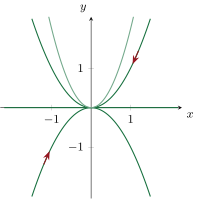
Consider $y' = 2\sqrt{\abs y}$ with $y(0) = 0$ . The zero function solves it; so does

y(t) = \begin{cases} 0 & t \leq 0,\\ t^2 & t \geq 0, \end{cases}

which is $C^1$ (both pieces have derivative $0$ at the glue point) and satisfies $y'(t) = 2t = 2\sqrt{t^2}$ for $t > 0$ — indeed, delaying the take-off gives a solution for every release time $c \geq 0$ : infinitely many solutions through the same initial data. No contradiction with Theorem 16.1: near $y = 0$ ,

\frac{\abs{2\sqrt y - 2\sqrt z}}{\abs{y - z}} = \frac{2}{\sqrt y + \sqrt z} \longrightarrow +\infty ,

the field is not Lipschitz in $y$ , and the theorem is silent. Closing insight: the physical reading is a bucket draining under gravity run backwards — from the empty state, one cannot tell when it started filling; determinism of ODEs is exactly the Lipschitz condition, not a law of nature.

16.2 Linear systems

Theorem 16.4 (Structure of linear systems)

Let $A \colon I \to \mathcal{M}_n(\R)$ and $B \colon I \to \R^n$ be continuous on an interval $I$ . For every $(t_0, X_0)$ the problem

X' = A(t)X + B(t), \qquad X(t_0) = X_0

has exactly one solution on all of $I$ . The solutions of the homogeneous system ( $B = 0$ ) form a vector space $\mathcal{S}_H$ of dimension exactly $n$ , and evaluation $X \mapsto X(t_0)$ is an isomorphism $\mathcal{S}_H \to \R^n$ ; general solution $=$ particular $+$ homogeneous.

Proof. On every segment $J \subseteq I$ containing $t_0$ : $f(t, X) = A(t)X + B(t)$ is continuous, and Lipschitz in $X$ with constant $k = \sup_J \vertiii{A(t)}$ (finite: continuous on a segment): Theorem 16.1 applies on $J$ ; letting $J$ exhaust $I$ , uniqueness glues the solutions into one on $I$ . Linearity of the solution set and of the evaluation map are clear; evaluation is bijective by existence (surjective) and uniqueness (injective): $\dim \mathcal{S}_H = n$ . The affine structure is Year 1’s argument verbatim. ∎

Example 16.5 (The evaluation isomorphism, concretely)

For $y'' + y = 0$ , viewed as the system $X' = \begin{pmatrix} 0 & 1\\ -1 & 0\end{pmatrix}X$ with $X = (y, y')$ : the theorem says the solution space is a plane, and that $X \mapsto X(0) = (y(0), y'(0))$ is an isomorphism onto $\R^2$ . The solutions $\cos$ and $\sin$ evaluate to $(1, 0)$ and $(0, 1)$ — the canonical basis of $\R^2$ — so they form a basis of the solution space, and every solution is

y(t) = y(0)\cos t + y'(0)\sin t ,

with the coefficients read directly off the initial data, no linear system to solve. Closing insight: choosing the fundamental system whose initial values are the canonical basis (here $\cos, \sin$ ) is exactly choosing the columns of $\eu^{tA}$ ; the evaluation isomorphism is why initial conditions parametrize trajectories — the geometric content of “deterministic dynamics” for linear equations.

Definition 16.6 (Wronskian)

For solutions $X_1, \dots, X_n$ of the homogeneous system, the wronskian is $W(t) = \det\bigl(X_1(t), \dots, X_n(t)\bigr)$ . By the isomorphism above, either $W$ vanishes identically (the family is linked) or never (a fundamental system); quantitatively, $W' = \operatorname{tr}\bigl(A(t)\bigr) W$ , so

W(t) = W(t_0)\,\exp\Bigl(\int_{t_0}^{t} \operatorname{tr} A(s)\,\dd s\Bigr) \quad \text{(Liouville's formula)}.

Example 16.7 (Liouville checked on an Euler equation)

On $\intoo{0}{\infty}$ , the equation $t^2y'' + ty' - y = 0$ has the solutions $y_1(t) = t$ and $y_2(t) = \frac1t$ (substitute). Their wronskian:

W(t) = \det\begin{pmatrix} t & \tfrac1t\\[2pt] 1 & -\tfrac{1}{t^2}\end{pmatrix} = -\frac1t - \frac1t = -\frac2t ,

never zero: a fundamental system. Now check Liouville: in normalized form $y'' + \frac1t\,y' - \frac{1}{t^2}\,y = 0$ , the companion matrix $A(t) = \begin{pmatrix} 0 & 1\\ \frac{1}{t^2} & -\frac1t\end{pmatrix}$ has trace $-\frac1t$ , so

W(t) = W(1)\exp\Bigl(-\int_1^t\frac{\dd s}{s}\Bigr) = -2\,\eu^{-\ln t} = -\frac2t . \checkmark

Closing insight: Liouville predicts the shape of the wronskian before any solution is known — here, that $W$ must be $\frac{c}{t}$ ; this is what powers the reduction-of-order method (Proposition 16.15), where knowing $y_1$ and the wronskian’s form determines $y_2$ by one quadrature.

Proof of Liouville’s formula. $W(t) = \det M(t)$ with $M' = AM$ . Differentiating the determinant as a multilinear function of the columns,

W'(t) = \sum_j \det(X_1, \dots, X_j', \dots, X_n) = \sum_j \det(X_1, \dots, AX_j, \dots, X_n) .

Now the map $(C_1, \dots, C_n) \mapsto \sum_j \det(C_1, \dots, AC_j, \dots, C_n)$ is $n$ -linear and alternating (with two equal columns $C_i = C_k$ , the terms $j \notin \{i, k\}$ vanish outright, and the terms $j = i$ and $j = k$ cancel in pairs after one column swap): by the uniqueness theorem (Theorem 2.14) it is $c \cdot \det$ , with $c$ read on the canonical columns: $c = \sum_j \det(e_1, \dots, Ae_j, \dots, e_n) = \sum_j a_{jj} = \operatorname{tr} A$ . Hence $W' = \operatorname{tr}\bigl(A(t)\bigr)W$ : a scalar linear ODE, solved by the Year 1 formula. ∎

16.3 Constant coefficients: the matrix exponential

Theorem 16.8

For $A \in \mathcal{M}_n(\R)$ (or $\C$ ), the exponential $\eu^{tA} = \sum_k \frac{(tA)^k}{k!}$ (Example 5.22) satisfies: $t \mapsto \eu^{tA}$ is $C^1$ (indeed $C^\infty$ ) with

\frac{\dd}{\dd t}\,\eu^{tA} = A\,\eu^{tA} = \eu^{tA}A , \qquad \eu^{(s+t)A} = \eu^{sA}\,\eu^{tA}, \qquad (\eu^{A})^{-1} = \eu^{-A} ;

and $\eu^{A + B} = \eu^A\eu^B$ when $AB = BA$ . The Cauchy problem $X' = AX$ , $X(0) = X_0$ has the unique solution $X(t) = \eu^{tA}X_0$ ; with a source, the variation of constants formula holds:

X(t) = \eu^{(t - t_0)A}X_0 + \int_{t_0}^{t} \eu^{(t-s)A}B(s)\,\dd s .

Proof. Differentiability: the series $\sum \frac{t^kA^k}{k!}$ and its term-derived series $\sum \frac{t^{k-1}A^k}{(k-1)!} = A\sum \frac{(tA)^{k-1}}{(k-1)!}$ converge normally on every segment (norms $\leq \frac{(\abs t\,\vertiii A)^k}{k!}$ ): differentiate term by term (Theorem 10.11, vector-valued). The two orderings $A\eu^{tA}$ and $\eu^{tA}A$ agree since every partial sum commutes with $A$ .

Group law: for commuting $A, B$ , the Cauchy product of the two exponential series reorganizes by the binomial theorem exactly as in Example 7.15 (absolute convergence in the Banach algebra justifies it): $\eu^{A+B} = \eu^A\eu^B$ ; with $B = sA$ this gives the one-parameter group law, and $B = -A$ the inverse.

Cauchy problem: $X(t) = \eu^{tA}X_0$ solves it (differentiate); uniqueness by Theorem 16.4. Variation of constants: set $Y(t) = \eu^{-tA}X(t)$ ; differentiating, $Y' = \eu^{-tA}(X' - AX) = \eu^{-tA}B(t)$ ; integrate from $t_0$ to $t$ and multiply back by $\eu^{tA}$ . ∎

Method 16.9 (Computing $\eu^{tA}$ )

Reduce $A$ (Chapter 3): if $A = PDP^{-1}$ diagonal, $\eu^{tA} = P\,\eu^{tD}P^{-1}$ with $\eu^{tD}$ diagonal of $\eu^{t\lambda_i}$ ; in general use Dunford $A = D + N$ (commuting): $\eu^{tA} = \eu^{tD}\,\eu^{tN}$ with $\eu^{tN}$ a polynomial in $t$ (nilpotence truncates the series). Complex eigenvalues pair into rotation-times-exponential blocks (Exercise 16.5).

Remark 16.10 (Common pitfalls)

(i) $\eu^{A+B} \neq \eu^A\eu^B$ without commutation: take $A = \begin{pmatrix} 0 & 1\\ 0 & 0\end{pmatrix}$ , $B = \begin{pmatrix} 0 & 0\\ 1 & 0\end{pmatrix}$ . Then $\eu^A = I + A$ , $\eu^B = I + B$ (nilpotence), so

\eu^A\eu^B = \begin{pmatrix} 2 & 1\\ 1 & 1\end{pmatrix}, \qquad\text{while}\qquad \eu^{A+B} = \cosh(1)\,I + \sinh(1)\,(A + B) = \begin{pmatrix} \cosh 1 & \sinh 1\\ \sinh 1 & \cosh 1 \end{pmatrix},

using $(A+B)^2 = I$ ; and $\cosh 1 \approx 1.54 \neq 2$ . The group law of Theorem 16.8 carries a genuine hypothesis. (ii) Nonlinear intuition on linear turf: solutions of a linear system with continuous coefficients live on the whole interval (Theorem 16.4) — if a candidate solution explodes inside $I$ , the equation was not linear or the computation is wrong; conversely, for nonlinear equations never promise globality without an argument ( $y' = y^2$ ). (iii) Dividing by the unknown: separating variables in $y' = y(1-y)$ silently discards the constant solutions $0$ and $1$ — exactly the ones that organize the phase line (Exercise 16.3); list constant solutions first. (iv) Initial data fix vectors, not scalars: an $n$ -th order scalar equation needs $n$ conditions ( $y, y', \dots$ at $t_0$ ); matching only $y(t_0)$ leaves an $(n-1)$ -parameter family, a classic source of “lost” constants.

Example 16.11 (A $3\times3$ exponential by Dunford)

Solve $X' = AX$ for $A = \begin{pmatrix} 2 & 1 & 0\\ 0 & 2 & 0\\ 0 & 0 & 3\end{pmatrix}$ . Dunford by blocks: $A = D + N$ with $D = \operatorname{diag}(2, 2, 3)$ and $N = E_{12}$ , which commute ( $N$ lives inside the eigenvalue- $2$ block), and $N^2 = 0$ :

\eu^{tA} = \eu^{tD}\,\eu^{tN} = \begin{pmatrix} \eu^{2t} & t\,\eu^{2t} & 0\\ 0 & \eu^{2t} & 0\\ 0 & 0 & \eu^{3t} \end{pmatrix} .

The general solution reads off column by column: $X(t) = \bigl(\eu^{2t}(x_0 + ty_0),\ \eu^{2t}y_0,\ \eu^{3t}z_0\bigr)$ . Sanity checks: at $t = 0$ the matrix is $I$ ; its determinant is $\eu^{7t} = \eu^{t\operatorname{tr}A}$ , as Liouville demands; and the factor $t$ appears exactly where the eigenvalue $2$ is defective. Closing insight: polynomials times exponentials are not a guess to be memorized — they are the truncated series $\eu^{tN}$ , and their degree is bounded by the nilpotency index, never more.

Method 16.12 (Solving $X' = AX + B(t)$ , start to finish)

Spectrum of $A$ ; then $\eu^{tA}$ by Method 16.9 (diagonalize; or Dunford as in Example 16.11; or a polynomial trick like $A^2 = -I$ ).
A particular solution: variation of constants $\int_{t_0}^t\eu^{(t-s)A}B(s)\dd s$ always works; for exponential-polynomial $B$ , an ansatz of the same shape (degree raised on resonance, Exercise 16.10) is faster.
General solution $= \eu^{(t-t_0)A}X_0 +$ particular; fit the initial data last, on the complete formula.
Sanity checks: $X(t_0)$ correct; the homogeneous part’s growth matches the eigenvalue real parts (Exercise 16.8); and $\det$ of a fundamental matrix obeys Liouville.

Example 16.13 (A phase portrait)

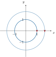
$X' = AX$ with $A = \begin{pmatrix} 0 & 1\\ -1 & 0\end{pmatrix}$ : $A^2 = -I$ , so the series splits into

\eu^{tA} = (\cos t)\,I + (\sin t)\,A = \begin{pmatrix} \cos t & \sin t\\ -\sin t & \cos t \end{pmatrix} :

trajectories are circles run clockwise — the harmonic oscillator $x'' + x = 0$ in first-order clothes. Eigenvalues $\pm\iu$ on the imaginary axis: a center. More generally the real parts of the eigenvalues of $A$ decide growth or decay of $\norm{X(t)}$ (Exercise 16.8).

Two linear phase portraits. Left: a center (eigenvalues ±) — closed circular orbits of the harmonic oscillator. Right: a stable node (eigenvalues -1, -2) — all trajectories fall into the origin tangentially to the slow eigendirection. — Two linear phase portraits. Left: a *center* (eigenvalues $\pm\iu$ ) — closed circular orbits of the harmonic oscillator. Right: a *stable node* (eigenvalues $-1, -2$ ) — all trajectories fall into the origin tangentially to the slow eigendirection.

The trace–determinant plane for X' = AX in dimension 2: below the horizontal axis, saddles; between the axis and the parabola = 2/4, nodes; inside the parabola, spirals; on the positive -axis, centers. The weekend problem proves this classification and follows one vertical line of it — the damped oscillator — into resonance. — The trace–determinant plane for $X' = AX$ in dimension $2$ : below the horizontal axis, saddles; between the axis and the parabola $\delta = \tau^2/4$ , nodes; inside the parabola, spirals; on the positive $\delta$ -axis, centers. The weekend problem proves this classification and follows one vertical line of it — the damped oscillator — into resonance.

Remark 16.14 (Where this is used)

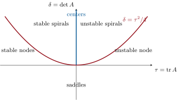
Linear systems are the local model for everything nonlinear: near an equilibrium, a smooth vector field behaves (in the hyperbolic cases) like its linearization, whose portrait the trace–determinant plane classifies. The weekend problem works out the oscillator story in full — damping, forcing, resonance, and Sturm’s comparison theorems for variable coefficients — the mathematics behind shock absorbers, AC circuits, and spectral gaps alike. The Year 3 volume returns with the qualitative theory (flows, stability, first integrals) on manifolds.

16.4 Second order with variable coefficients

Proposition 16.15

The equation $y'' + a(t)y' + b(t)y = c(t)$ ( $a, b, c$ continuous on $I$ ) is the system $X' = A(t)X + B(t)$ for $X = (y, y')$ : solutions exist and are unique on all of $I$ for any initial data $(y(t_0), y'(t_0))$ ; homogeneous solutions form a plane. If one nonvanishing homogeneous solution $y_1$ is known, a second independent one is found by lowering the order: setting $y = y_1 z$ turns the homogeneous equation into a first-order equation for $z'$ , solved by quadratures.

Proof. The system form and Theorem 16.4 give everything structural. Lowering: substituting $y = y_1z$ ,

y_1 z'' + (2y_1' + a y_1)z' + \underbrace{(y_1'' + ay_1' + by_1)}_{=\,0}\,z = 0 :

a first-order linear equation in $u = z'$ , solvable by the Year 1 formula; integrating $u$ gives $z$ , hence $y_2 = y_1 z$ , independent of $y_1$ whenever $z$ is nonconstant. ∎

Example 16.16

$t^2y'' - 2y = 0$ on $\intoo{0}{\infty}$ : $y_1 = t^2$ is a solution. Substitute $y = t^2z$ : from $y' = t^2z' + 2tz$ and $y'' = t^2z'' + 4tz' + 2z$ ,

t^2y'' - 2y = t^4 z'' + 4t^3z' = 0, \qquad\text{i.e.}\qquad \frac{z''}{z'} = -\frac4t :

$z' = t^{-4}$ (up to a constant), $z = -\frac{1}{3t^3}$ , and $y_2 = t^2z = -\frac{1}{3t}$ . General solution: $y = \alpha t^2 + \frac{\beta}{t}$ .

16.5 Exercises

Exercise 16.1 ★

Solve $X' = AX$ , $X(0) = (1, 0)^{\mathsf T}$ , for $A = \begin{pmatrix} 1 & 1\\ 0 & 2\end{pmatrix}$ (diagonalize) and $A = \begin{pmatrix} 2 & 1\\ 0 & 2 \end{pmatrix}$ (Dunford).

Solution

Solution of Exercise 16.1.

First matrix: eigenvalues $1, 2$ , eigenvectors $(1,0)$ and $(1,1)$ . Decompose $X_0 = (1,0) = 1\cdot(1,0) + 0\cdot(1,1)$ : the solution is

X(t) = \eu^{t}\begin{pmatrix}1\\ 0\end{pmatrix} .

(The initial vector is itself an eigenvector.)

Second: $A = 2I + N$ , $N = E_{12}$ , $N^2 = 0$ : $\eu^{tA} = \eu^{2t}(I + tN)$ , so

X(t) = \eu^{2t}\begin{pmatrix} 1 & t\\ 0 & 1\end{pmatrix} \begin{pmatrix}1\\ 0\end{pmatrix} = \eu^{2t}\begin{pmatrix}1\\ 0\end{pmatrix}.

Exercise 16.2 ★

Which Cauchy problems have unique global solutions on $\R$ by Theorem 16.1? $y' = \sin(ty)$ ; $\;y' = y^2$ ; $\;y' = \abs y$ . For the last, solve explicitly with $y(0) = 0$ and $y(0) = 1$ .

Solution

Solution of Exercise 16.2.

$y' = \sin(ty)$ : $\abs{\sin(ty) - \sin(tz)} \leq \abs t\,\abs{y - z}$ — Lipschitz in $y$ uniformly on every segment of times: unique global solutions on $\R$ (apply the theorem on every segment).

$y' = y^2$ : locally Lipschitz only; no global theorem, and indeed $y(0) = 1$ explodes at $t = 1$ .

$y' = \abs y$ : $\abs\cdot$ is $1$ -Lipschitz: global existence and uniqueness. With $y(0) = 0$ : $y \equiv 0$ (uniqueness!). With $y(0) = 1$ : $y$ stays positive (cannot cross the zero solution), so $y' = y$ : $y = \eu^t$ .

Exercise 16.3 ★

Prove that two distinct maximal solutions of $y' = f(t,y)$ ( $f$ Lipschitz in $y$ ) never take the same value at the same time, and deduce that solutions of $y' = y(1 - y)$ starting in $\intoo{0}{1}$ remain in $\intoo{0}{1}$ forever.

Solution

Solution of Exercise 16.3.

If $y(t_1) = z(t_1)$ at some time, then $y$ and $z$ solve the same Cauchy problem at $t_1$ : uniqueness forces $y = z$ on their common interval — distinct solutions never meet.

For $y' = y(1-y)$ : the constants $0$ and $1$ are solutions. A solution starting in $\intoo{0}{1}$ can never reach $0$ or $1$ (it would collide with a constant solution): it stays in $\intoo{0}{1}$ , hence is global (bounded: no explosion — e.g. by Exercise 16.9’s criterion, or because the vector field is bounded on the trapped strip).

Exercise 16.4 ★★

Compute $\eu^{tA}$ for $A = \begin{pmatrix} 3 & 1\\ -1 & 1\end{pmatrix}$ (Dunford: $(A - 2I)^2 = 0$ ), and solve $X' = AX + \begin{pmatrix} \eu^{2t}\\ 0\end{pmatrix}$ , $X(0) = 0$ , by variation of constants.

Solution

Solution of Exercise 16.4.

$(A - 2I)^2 = \begin{pmatrix}1 & 1\\ -1 & -1\end{pmatrix}^2 = 0$ : Dunford with $D = 2I$ , $N = A - 2I$ :

\eu^{tA} = \eu^{2t}\,(I + tN) = \eu^{2t}\begin{pmatrix} 1 + t & t\\ -t & 1 - t\end{pmatrix}.

Variation of constants with $B(s) = (\eu^{2s}, 0)^{\mathsf T}$ :

X(t) = \int_0^t \eu^{(t-s)A}B(s)\,\dd s = \eu^{2t}\int_0^t \begin{pmatrix} 1 + (t-s)\\ -(t-s) \end{pmatrix}\dd s = \eu^{2t}\begin{pmatrix} t + \frac{t^2}{2}\\[2pt] -\frac{t^2}{2} \end{pmatrix},

using $\eu^{(t-s)A}B(s) = \eu^{2(t-s)}(I + (t-s)N)\,(\eu^{2s}, 0)^{\mathsf T} = \eu^{2t}\bigl(1 + (t-s),\, -(t-s)\bigr)^{\mathsf T}$ . (Check: $X(0) = 0$ ; $X' - AX = (\eu^{2t}, 0)^{\mathsf T}$ by differentiation.)

Exercise 16.5 ★★

For $A = \begin{pmatrix} \alpha & -\beta\\ \beta & \alpha\end{pmatrix}$ , prove $\eu^{tA} = \eu^{\alpha t}\begin{pmatrix} \cos\beta t & -\sin\beta t\\ \sin\beta t & \cos\beta t\end{pmatrix}$ — spiral trajectories — two ways: via the series (write $A = \alpha I + \beta J$ , $J^2 = -I$ ), and via the complex identification $z' = (\alpha + \iu\beta)z$ .

Solution

Solution of Exercise 16.5.

Series: $A = \alpha I + \beta J$ with $J = \begin{pmatrix}0 & -1\\ 1 & 0\end{pmatrix}$ , $J^2 = -I$ ; the two summands commute, so $\eu^{tA} = \eu^{\alpha t}\,\eu^{\beta tJ}$ , and the series of $\eu^{\beta t J}$ splits along even/odd powers into $\cos(\beta t)I + \sin(\beta t)J$ : the stated rotation-scaling matrix.

Complex: identify $(x, y) \in \R^2$ with $z = x + \iu y$ ; the system $X' = AX$ reads $z' = (\alpha + \iu\beta)z$ , whose solution $z(t) = \eu^{\alpha t}\eu^{\iu\beta t}z_0$ is exactly the spiral: modulus $\eu^{\alpha t}$ , argument advancing at speed $\beta$ .

Exercise 16.6 ★★

(Gronwall’s lemma) Let $u$ be continuous nonnegative with $u(t) \leq C + k\int_{t_0}^{t} u(s)\,\dd s$ on $\intco{t_0}{T}$ . Prove $u(t) \leq C\,\eu^{k(t - t_0)}$ (differentiate $v(t) = \eu^{-kt}\int_{t_0}^t u$ ). Deduce again the uniqueness in Cauchy–Lipschitz and the continuous dependence $\norm{y(t) - z(t)} \leq \norm{y_0 - z_0}\,\eu^{k\abs{t - t_0}}$ for two solutions with different initial data.

Solution

Solution of Exercise 16.6.

Let $v(t) = \eu^{-k(t - t_0)}\int_{t_0}^t u$ . Then

v'(t) = \eu^{-k(t-t_0)}\Bigl(u(t) - k\int_{t_0}^t u\Bigr) \leq C\,\eu^{-k(t-t_0)},

by the hypothesis. Integrating from $t_0$ to $t$ ( $v(t_0) = 0$ ): $v(t) \leq \frac{C}{k}\bigl(1 - \eu^{-k(t - t_0)}\bigr)$ , i.e. $k\int_{t_0}^t u \leq C\bigl(\eu^{k(t-t_0)} - 1\bigr)$ ; feeding this back into the hypothesis: $u(t) \leq C\eu^{k(t-t_0)}$ .

Uniqueness/dependence: two solutions $y, z$ of the integral equation satisfy

\norm{y(t) - z(t)} \leq \norm{y_0 - z_0} + k\int_{t_0}^{t}\norm{y - z},

and Gronwall with $C = \norm{y_0 - z_0}$ gives the exponential bound; $C = 0$ gives uniqueness.

Exercise 16.7 ★★

Knowing that $y_1(t) = \frac{\sin t}{t}$ solves $ty'' + 2y' + ty = 0$ on $\intoo{0}{\pi}$ , find a second independent solution by lowering the order, and give the general solution.

Solution

Solution of Exercise 16.7.

Substitute $y = y_1 z$ with $y_1 = \frac{\sin t}{t}$ : the general lowering formula (Proposition 16.15) gives, for $u = z'$ ,

y_1 u' + \Bigl(2y_1' + \frac{2}{t}\,y_1\Bigr)u = 0

(the equation normalized as $y'' + \frac2t y' + y = 0$ ). Compute $2y_1' + \frac2t y_1 = 2\,\frac{t\cos t - \sin t}{t^2} + \frac{2\sin t}{t^2} = \frac{2\cos t}{t}$ : so

\frac{u'}{u} = -\frac{2\cos t}{t}\cdot\frac{t}{\sin t} = -2\cot t \quad\Longrightarrow\quad u = \frac{1}{\sin^2 t} \quad (\text{up to a constant}),

and $z = -\cot t$ , giving $y_2 = y_1 z = -\frac{\cos t}{t}$ . General solution on $\intoo{0}{\pi}$ :

y(t) = \alpha\,\frac{\sin t}{t} + \beta\,\frac{\cos t}{t} .

(These are the spherical Bessel functions of order zero.)

Exercise 16.8 ★★★

Let $A \in \mathcal{M}_n(\C)$ with all eigenvalues of (strictly) negative real part. Prove that every solution of $X' = AX$ tends to $0$ as $t \to +\infty$ , with an exponential rate: $\norm{X(t)} \leq C\,\eu^{-\alpha t}$ for some $\alpha > 0$ . (Trigonalize; treat the triangular system from the last row up, or use Dunford: $\eu^{tA} = \eu^{tD}\eu^{tN}$ with $\norm{\eu^{tD}} \leq \eu^{-\alpha' t}$ and $\eu^{tN}$ polynomial in $t$ .)

Solution

Solution of Exercise 16.8.

Dunford: $A = D + N$ commuting, $D$ diagonalizable with the same eigenvalues, $N$ nilpotent, so

\eu^{tA} = \eu^{tD}\,\eu^{tN}, \qquad \eu^{tN} = \sum_{k < n} \frac{t^kN^k}{k!} \ \text{(a matrix polynomial in } t).

Let $-2\alpha = \max_i \Re\lambda_i < 0$ . In a basis diagonalizing $D$ , $\vertiii{\eu^{tD}} \leq \eu^{-2\alpha t}$ (entries $\eu^{t\lambda_i}$ of modulus $\eu^{t\Re\lambda_i}$ ); norms in different bases differ by constants. Hence

\norm{X(t)} \leq \vertiii{\eu^{tA}}\,\norm{X_0} \leq C'\,\eu^{-2\alpha t}\,(1 + t)^{n-1}\,\norm{X_0} \leq C\,\eu^{-\alpha t}\norm{X_0} ,

absorbing the polynomial into one exponential factor ( $\eu^{-\alpha t}(1+t)^{n-1} \to 0$ , hence bounded).

Exercise 16.9 ★★★

(No escape in finite time for linear growth) Suppose $f$ is continuous with $\norm{f(t, y)} \leq a\norm y + b$ on $\intco{0}{\infty} \times \R^n$ , locally Lipschitz in $y$ . Using Gronwall (Exercise 16.6) on the integral form, prove that maximal solutions are global (defined on all of $\intco{0}{\infty}$ ).

Solution

Solution of Exercise 16.9.

Let $y$ be a maximal solution on $\intco{0}{T}$ , $T \leq \infty$ , and suppose $T < \infty$ . The integral form gives, for $t < T$ ,

\norm{y(t)} \leq \norm{y_0} + \int_0^t \bigl(a\norm{y(s)} + b\bigr)\dd s \leq \bigl(\norm{y_0} + bT\bigr) + a\int_0^t\norm{y(s)}\,\dd s ,

and Gronwall bounds $\norm{y(t)} \leq (\norm{y_0} + bT)\,\eu^{aT} =: M$ on $\intco{0}{T}$ : the solution stays in a compact ball. Then $y' = f(t, y)$ is bounded near $T$ , so $y$ is Lipschitz near $T$ and extends continuously to $T$ (Cauchy criterion); solving the Cauchy problem at $(T, y(T))$ prolongs $y$ beyond $T$ , contradicting maximality. Hence $T = \infty$ : no finite-time escape under linear growth.

Exercise 16.10 ★

Solve $y'' - 3y' + 2y = \eu^{t}$ : homogeneous solutions, then a particular solution of the form $\alpha t\,\eu^{t}$ (why does the naive guess $\alpha\eu^t$ fail?); general solution and the solution with $y(0) = y'(0) = 0$ .

Solution

Solution of Exercise 16.10.

Characteristic roots of $r^2 - 3r + 2$ : $1$ and $2$ , so the homogeneous solutions are $a\eu^t + b\eu^{2t}$ . The guess $\alpha\eu^t$ fails because $\eu^t$ already solves the homogeneous equation (the root $r = 1$ “resonates” with the right-hand side). With $y = \alpha t\,\eu^t$ : $y' = \alpha(1 + t)\eu^t$ , $y'' = \alpha(2 + t)\eu^t$ , and

y'' - 3y' + 2y = \alpha\eu^t\bigl(2 + t - 3 - 3t + 2t\bigr) = -\alpha\,\eu^t :

$\alpha = -1$ , $y_p = -t\,\eu^t$ . General solution: $y = a\eu^t + b\eu^{2t} - t\eu^t$ . Initial data $y(0) = y'(0) = 0$ : $a + b = 0$ and $a + 2b - 1 = 0$ : $b = 1$ , $a = -1$ :

y(t) = \eu^{2t} - (1 + t)\,\eu^{t} .

Exercise 16.11 ★★

Compute $\eu^{tA}$ for the Jordan block

A = \begin{pmatrix} \lambda & 1 & 0\\ 0 & \lambda & 1\\ 0 & 0 & \lambda\end{pmatrix},

and describe all solutions of $X' = AX$ : exponentials times polynomial vectors, with degrees up to $2$ . Where does the polynomial degree come from?

Solution

Solution of Exercise 16.11.

$A = \lambda I + N$ with $N = E_{12} + E_{23}$ : $N^2 = E_{13}$ , $N^3 = 0$ , and $\lambda I$ commutes with $N$ :

\eu^{tA} = \eu^{\lambda t}\Bigl(I + tN + \frac{t^2}{2}N^2\Bigr) = \eu^{\lambda t}\begin{pmatrix} 1 & t & \frac{t^2}{2}\\ 0 & 1 & t\\ 0 & 0 & 1 \end{pmatrix}.

Solutions: $X(t) = \eu^{\lambda t}\bigl(X_0 + tNX_0 + \frac{t^2}2N^2X_0\bigr)$ — each component is $\eu^{\lambda t}$ times a polynomial of degree $\leq 2$ . The degree bound is the nilpotency index minus one: the series of $\eu^{tN}$ truncates at $N^2$ .

Exercise 16.12 ★★★

(Periodic forcing, periodic response) Let $A \in \mathcal{M}_n(\R)$ and $B \colon \R \to \R^n$ continuous and $T$ -periodic.

Show that a solution of $X' = AX + B(t)$ is $T$ -periodic if and only if $X(T) = X(0)$ (compare $X(\cdot + T)$ and $X$ ).
Show that eigenvalues of $\eu^{TA}$ are the $\eu^{T\lambda}$ , $\lambda \in \operatorname{Sp}A$ (trigonalize over $\C$ ). Deduce: if no eigenvalue of $A$ lies in $\frac{2\iu\pi}{T}\Z$ , then $I - \eu^{TA}$ is invertible.
Under that hypothesis, prove that the system has exactly one $T$ -periodic solution, with

$X(0) = \bigl(I - \eu^{TA}\bigr)^{-1} \int_0^{T}\eu^{(T-s)A}B(s)\,\dd s .$

What does the excluded case correspond to, for the harmonic oscillator? (The weekend problem answers: resonance.)

Solution

Solution of Exercise 16.12.

If $X(T) = X(0)$ , then $Y(t) = X(t + T)$ solves $Y' = AY + B(t + T) = AY + B(t)$ with $Y(0) = X(0)$ : uniqueness (Theorem 16.4) gives $Y = X$ , i.e. $X$ is $T$ -periodic. The converse is trivial.
Trigonalize over $\C$ : $A = PT'P^{-1}$ with $T'$ upper triangular, diagonal $(\lambda_i)$ . Every power of a triangular matrix is triangular with diagonal $(\lambda_i^k)$ , so $\eu^{TA} = P\eu^{TT'}P^{-1}$ is triangular in the same basis with diagonal $(\eu^{T\lambda_i})$ : those are the eigenvalues. Then $I - \eu^{TA}$ is invertible iff $\eu^{T\lambda} \neq 1$ for every eigenvalue, i.e. iff $T\lambda \notin 2\iu\pi\Z$ , which is the stated hypothesis.
Variation of constants: $X(T) = \eu^{TA}X(0) + \int_0^T\eu^{(T-s)A}B(s)\dd s$ , so $X(T) = X(0)$ reads

$\bigl(I - \eu^{TA}\bigr)X(0) = \int_0^{T}\eu^{(T-s)A}B(s)\,\dd s ,$

which has a unique solution $X(0)$ under the invertibility hypothesis: exactly one $T$ -periodic solution. For the harmonic oscillator ( $\lambda = \pm\iu\omega$ ), the excluded case is $\omega T \in 2\pi\Z$ : forcing whose period is a multiple of the natural period — resonance, as the weekend problem quantifies.

16.6 Problem: Oscillations, resonance, and Sturm’s comparison theorems

Problem 16.1

One equation rules the mechanical and electrical world:

x'' + 2\zeta\omega\,x' + \omega^2 x = F(t), \qquad \omega > 0,\ \zeta \geq 0 .

This problem studies it completely — via the trace–determinant classification of planar linear systems, the three damping regimes, the steady-state response to periodic forcing with its resonance peak and the resonance catastrophe — then leaves constant coefficients for Sturm’s separation and comparison theorems, which control the zeros of solutions of $y'' + q(t)y = 0$ with no formula at all.

Part I — The trace–determinant plane. Let $A \in \mathcal M_2(\R)$ , $\tau = \operatorname{tr}A$ , $\delta = \det A$ , $\Delta = \tau^2 - 4\delta$ .

Show that the eigenvalues of $A$ are $\frac{\tau\pm\sqrt\Delta}{2}$ and classify: two real eigenvalues of opposite signs iff $\delta < 0$ ; real eigenvalues of the same sign iff $\delta > 0$ , $\Delta \geq 0$ (sign of $\tau$ ); nonreal conjugate pair iff $\Delta < 0$ (real part $\frac\tau2$ ).
(Saddle, $\delta < 0$ ) With eigenvalues $\mu < 0 < \lambda$ and eigenvectors $v_\pm$ , write the general solution and describe the trajectories: two stable and two unstable rays, all other orbits asymptotic to both. Why can no solution but $0$ stay bounded on all of $\R$ ?
(Nodes, $\delta > 0$ , $\Delta > 0$ ) For $\mu < \lambda < 0$ : show every nonzero solution tends to $0$ and that all orbits except those on the fast axis arrive tangent to the slow eigendirection (compare $\eu^{\mu t}$ and $\eu^{\lambda t}$ ).
(Spirals and centers, $\Delta < 0$ ) Writing the eigenvalues $\alpha \pm \iu\beta$ , use Exercise 16.5 (after a real change of basis, admitted in that generality or proved for the systems of Part II, which are the ones used below) to describe the orbits: spirals converging for $\alpha = \frac\tau2 < 0$ , diverging for $\tau > 0$ , closed curves (center) for $\tau = 0$ .
(Boundary cases) For a double eigenvalue ( $\Delta = 0$ ): show $\eu^{tA} = \eu^{\lambda t}(I + tN)$ with $N = A - \lambda I$ nilpotent, and distinguish the star ( $N = 0$ ) from the improper node ( $N \neq 0$ ). Summarize Part I in the trace–determinant picture of this chapter’s figure.

Part II — The damped oscillator. Now $F = 0$ : $x'' + 2\zeta\omega x' + \omega^2x = 0$ , i.e. $X' = AX$ with $A = \begin{pmatrix} 0 & 1\\ -\omega^2 & -2\zeta\omega\end{pmatrix}$ .

Compute $\tau, \delta, \Delta$ and place the three regimes in the trace–determinant plane: underdamped $0 < \zeta < 1$ (stable spiral), critically damped $\zeta = 1$ (double eigenvalue), overdamped $\zeta > 1$ (stable node); $\zeta = 0$ is the center.
Solve the three regimes explicitly:

$\zeta < 1:\ \eu^{-\zeta\omega t}\bigl(a\cos\omega_d t + b\sin\omega_dt\bigr),\ \omega_d = \omega\sqrt{1-\zeta^2}; \qquad \zeta = 1:\ (a + bt)\,\eu^{-\omega t};$

$\zeta > 1$ : two real exponentials. Define the pseudo-period $\frac{2\pi}{\omega_d}$ and show that the ratio of successive maxima of $\abs x$ is the constant $\eu^{-2\pi\zeta/\sqrt{1-\zeta^2}}$ (the logarithmic decrement).
(The door-closer principle) For $\zeta \geq 1$ the decay rate is governed by the slowest eigenvalue $\lambda_{\mathrm{slow}} = -\omega\bigl(\zeta - \sqrt{\zeta^2-1}\bigr)$ . Show that $\abs{\lambda_{\mathrm{slow}}} = \frac{\omega}{\zeta + \sqrt{\zeta^2 - 1}}$ is a decreasing function of $\zeta \geq 1$ : critical damping $\zeta = 1$ gives the fastest non-oscillating return to rest.
(Energy) Let $E(t) = \frac12x'^2 + \frac12\omega^2x^2$ . Prove $E' = -2\zeta\omega\,x'^2 \leq 0$ , and deduce that for $\zeta > 0$ the equation has no nonzero periodic solution (a period would force $E$ constant, hence $x' \equiv 0$ ).
Explain in two sentences why the center $\zeta = 0$ is structurally fragile: any $\zeta > 0$ , however small, destroys periodicity — and where that shows in the trace–determinant plane (the center line has empty interior).

Part III — Forced oscillations and resonance. Now $F(t) = F\cos(\gamma t)$ with $F, \gamma > 0$ .

( $\zeta > 0$ : the steady state) Seek $x_p = \Re\bigl(z\,\eu^{\iu\gamma t}\bigr)$ : show

$z = \frac{F}{\omega^2 - \gamma^2 + 2\iu\zeta\omega\gamma}, \qquad A(\gamma) := \abs z = \frac{F}{\sqrt{(\omega^2 - \gamma^2)^2 + 4\zeta^2\omega^2\gamma^2}} ,$

and write $x_p = A(\gamma)\cos(\gamma t - \varphi)$ with $\tan\varphi = \frac{2\zeta\omega\gamma}{\omega^2-\gamma^2}$ .
Show that every solution is $x_p$ plus a transient from Part II, which tends to $0$ : whatever the initial data, the system locks onto the steady state — amplitude $A(\gamma)$ , phase lag $\varphi$ .
(The resonance curve) Maximize $A$ : show that $A(\gamma)$ has an interior maximum iff $\zeta < \frac{1}{\sqrt2}$ , at

$\gamma_* = \omega\sqrt{1 - 2\zeta^2}, \qquad A(\gamma_*) = \frac{F}{2\zeta\omega^2\sqrt{1-\zeta^2}} ,$

and that for small $\zeta$ the peak amplifies the static response $A(0) = \frac F{\omega^2}$ by the factor $\approx \frac{1}{2\zeta}$ .
( $\zeta = 0$ , off resonance) For $\gamma \neq \omega$ , show that the solution with $x(0) = x'(0) = 0$ is

$x(t) = \frac{F}{\omega^2 - \gamma^2}\bigl(\cos\gamma t - \cos\omega t\bigr) = \frac{2F}{\omega^2-\gamma^2} \sin\frac{(\omega-\gamma)t}{2} \sin\frac{(\omega+\gamma)t}{2} :$

bounded, with beats — a fast oscillation under a slow envelope — when $\gamma$ is close to $\omega$ .
( $\zeta = 0$ , resonance) For $\gamma = \omega$ , show that $x_p(t) = \frac{F}{2\omega}\,t\sin(\omega t)$ is a solution, and recover it as the limit of question 14 as $\gamma \to \omega$ : the amplitude grows linearly forever — the resonance catastrophe.
(Fourier link) A general periodic forcing decomposes into harmonics (the Fourier chapter); by linearity the steady state is the sum of the harmonic responses. For an undamped oscillator of frequency $\omega = 3$ forced by the square wave of Exercise 14.1-type (harmonics at all odd integers), which harmonic resonates? One sentence on why engineers fear square waves.

Part IV — Sturm’s theorems. Consider $y'' + q(t)\,y = 0$ on an interval $I$ , $q$ continuous. (Any equation $y'' + ay' + by = 0$ reduces to this normal form by the substitution $y = u\exp\bigl(-\frac12\int a\bigr)$ ; question 21 shows a variant of the trick in action.)

For two solutions $y_1, y_2$ , show that the wronskian $W = y_1y_2' - y_1'y_2$ is constant, zero iff the solutions are proportional; and that a nonzero solution has only simple, isolated zeros.
(Sturm separation) Let $y_1, y_2$ be independent solutions and $a < b$ two consecutive zeros of $y_1$ . Prove that $y_2$ vanishes exactly once in $\intoo{a}{b}$ (evaluate the constant $W$ at $a$ and $b$ : $W = y_1'y_2$ there, and $y_1'(a)$ , $y_1'(b)$ have opposite signs): zeros of independent solutions interlace.
(Sturm comparison) Let $q_1 \leq q_2$ on $I$ , $y \neq 0$ with $y'' + q_1y = 0$ , $z \neq 0$ with $z'' + q_2z = 0$ , and $a < b$ consecutive zeros of $y$ . Show that $z$ vanishes in $\intcc{a}{b}$ — strictly inside if $q_1 < q_2$ somewhere on $\intoo ab$ (if $z \neq 0$ on $\intoo ab$ , study $(yz' - y'z)' = (q_1 - q_2)yz$ with fixed signs for $y, z$ and compare the boundary values).
Deduce the spacing bounds: if $0 < m^2 \leq q(t) \leq M^2$ on $I$ , then any two consecutive zeros $a < b$ of a nonzero solution of $y'' + qy = 0$ satisfy

$\frac{\pi}{M} \;\leq\; b - a \;\leq\; \frac{\pi}{m}$

(compare with $u'' + M^2u = 0$ and $u'' + m^2u = 0$ , whose zeros are spaced $\frac\pi M$ and $\frac\pi m$ ). Check on the harmonic oscillator.
Transform $ty'' + 2y' + ty = 0$ (Exercise 16.7) by $u = ty$ into $u'' + u = 0$ , recover its solutions $\frac{\sin t}t$ , $\frac{\cos t}{t}$ instantly, and conclude that the zeros of every nonzero solution are spaced exactly $\pi$ : Sturm’s world view — zeros are controlled by the coefficient $q$ , formulas or not.

Part V — Duhamel and the boundedness frontier.

(Duhamel for the oscillator) Show that for continuous $F$ , the solution of $x'' + \omega^2x = F(t)$ with $x(0) = x'(0) = 0$ is

$x(t) = \frac1\omega\int_0^t\sin\bigl(\omega(t - s)\bigr)F(s)\,\dd s ,$

and re-derive the resonant solution of question 15 from it with $F(s) = F\cos(\omega s)$ (product-to-sum).
( $\zeta > 0$ : bounded input, bounded output) Show that for $\zeta > 0$ and any bounded continuous $F$ , every solution of the damped equation is bounded on $\intco{0}{\infty}$ (variation of constants plus the exponential decay $\vertiii{\eu^{tA}} \leq C\eu^{-\alpha t}$ of Exercise 16.8).
( $\zeta = 0$ ) Show that with no damping, bounded periodic forcing keeps all solutions bounded except exactly at resonance ( $\gamma = \omega$ , question 15 versus question 14): damping is what turns the boundedness frontier into uniform stability.
Synthesis. In one sentence each: (i) how the trace–determinant plane organizes Parts I–II and where forcing (Part III) leaves it; (ii) the physical meaning of $\gamma_*$ , $A(\gamma_*)$ and the factor $\frac1{2\zeta}$ ; (iii) what Sturm’s theorems say that explicit formulas cannot; (iv) which two results of this problem the rest of the book will quietly reuse (Liouville-constant wronskians; bounded-input stability).

Solution

Solution of Problem 16.1.

1. The characteristic polynomial is $\lambda^2 - \tau\lambda + \delta$ , with roots $\frac{\tau\pm\sqrt\Delta}{2}$ . If $\delta < 0$ then $\Delta = \tau^2 - 4\delta > 0$ and the two real roots have product $\delta < 0$ : opposite signs. If $\delta > 0$ and $\Delta \geq 0$ : real roots of product $> 0$ and sum $\tau$ : both of the sign of $\tau$ . If $\Delta < 0$ : conjugate pair $\alpha \pm \iu\beta$ with $\alpha = \frac\tau2$ , $\beta = \frac{\sqrt{-\Delta}}2$ .

2. $X(t) = a\,\eu^{\mu t}v_- + b\,\eu^{\lambda t}v_+$ . Orbits with $a = 0$ (resp. $b = 0$ ) run along the unstable (resp. stable) eigenline; all others have $\norm X \to \infty$ in both time directions, asymptotic to $\R v_+$ as $t \to +\infty$ and to $\R v_-$ as $t \to -\infty$ : the saddle picture. Boundedness on all of $\R$ forces $b = 0$ (else explosion at $+\infty$ ) and $a = 0$ (at $-\infty$ ): only the origin.

3. With $\mu < \lambda < 0$ , both exponentials decay: $X(t) \to 0$ . If $b \neq 0$ , factor $\eu^{\lambda t}$ :

X(t) = \eu^{\lambda t}\bigl(b\,v_\lambda + a\,\eu^{(\mu - \lambda)t}v_\mu\bigr), \qquad \eu^{(\mu-\lambda)t} \to 0 :

the direction of $X(t)$ tends to $\R v_\lambda$ , the slow eigendirection — all orbits but the fast axis arrive tangent to it (the right panel of the chapter’s phase portraits).

4. In the basis where $A = \begin{pmatrix} \alpha & -\beta\\ \beta & \alpha\end{pmatrix}$ (Exercise 16.5; for the oscillator systems of Part II this form is reached by an explicit real change of basis), the solution is $\eu^{\alpha t}$ times a rotation of angle $\beta t$ : logarithmic spirals, contracting when $\alpha = \frac\tau2 < 0$ , expanding when $\tau > 0$ , and closed curves (ellipses in the original coordinates) when $\tau = 0$ : the center.

5. $\Delta = 0$ gives the double eigenvalue $\lambda = \frac\tau2$ ; by Cayley–Hamilton (Theorem 3.21), $(A - \lambda I)^2 = 0$ , so $N = A - \lambda I$ is nilpotent, commutes with $\lambda I$ , and $\eu^{tA} = \eu^{\lambda t}(I + tN)$ . If $N = 0$ : $A = \lambda I$ , all rays are orbits (star node). If $N \neq 0$ : $X(t) = \eu^{\lambda t}(X_0 + tNX_0)$ , and for $NX_0 \neq 0$ the direction converges to the single eigendirection $\operatorname{im}N$ : improper node. This completes the trace–determinant picture.

6. $\tau = -2\zeta\omega$ , $\delta = \omega^2 > 0$ , $\Delta = 4\omega^2(\zeta^2 - 1)$ . So: $0 < \zeta < 1$ gives $\Delta < 0$ , $\tau < 0$ : stable spiral; $\zeta = 1$ : $\Delta = 0$ : degenerate stable node; $\zeta > 1$ : $\Delta > 0$ , $\tau < 0$ , $\delta > 0$ : stable node; $\zeta = 0$ : $\tau = 0$ , $\delta > 0$ : center. A vertical journey in the plane at $\delta = \omega^2$ .

7. Roots $r = -\zeta\omega \pm \omega\sqrt{\zeta^2-1}$ . For $\zeta < 1$ : $r = -\zeta\omega \pm \iu\omega_d$ , $\omega_d = \omega\sqrt{1-\zeta^2}$ :

x(t) = \eu^{-\zeta\omega t}\bigl(a\cos\omega_dt + b\sin\omega_dt\bigr) = R\,\eu^{-\zeta\omega t}\cos(\omega_dt - \varphi) .

For $\zeta = 1$ : $x = (a + bt)\eu^{-\omega t}$ . For $\zeta > 1$ : $x = a\eu^{r_-t} + b\eu^{r_+t}$ , both rates negative. Successive maxima of $\abs x$ in the underdamped case occur at times separated by the pseudo-period $\frac{2\pi}{\omega_d}$ (same phase of the cosine), and their ratio is $\eu^{-\zeta\omega\cdot2\pi/\omega_d} = \eu^{-2\pi\zeta/\sqrt{1-\zeta^2}}$ : the logarithmic decrement, a damping meter readable on an oscilloscope.

8. Rationalizing,

\abs{\lambda_{\mathrm{slow}}} = \omega\bigl(\zeta - \sqrt{\zeta^2-1}\bigr) = \frac{\omega}{\zeta + \sqrt{\zeta^2 - 1}} ,

whose denominator increases with $\zeta \geq 1$ : the decay rate is largest at $\zeta = 1$ , where it equals $\omega$ . An overdamped door closes without slamming but slowly; critical damping is the engineer’s optimum.

9. $E' = x'x'' + \omega^2xx' = x'\bigl(-2\zeta\omega x' - \omega^2x\bigr) + \omega^2xx' = -2\zeta\omega\,x'^2 \leq 0$ . If $x$ were periodic and nonconstant, $E$ would be periodic and nonincreasing, hence constant, forcing $x' \equiv 0$ : $x$ constant, and then $\omega^2x = 0$ : $x \equiv 0$ . So for $\zeta > 0$ the only periodic solution is rest: damping kills every cycle.

10. The center $\zeta = 0$ lives on the line $\tau = 0$ of the trace–determinant plane — a set with empty interior: an arbitrarily small perturbation of the matrix (any physical damping) moves $\tau$ off zero and turns the closed orbits into spirals. Periodicity of the undamped oscillator is thus a razor’s-edge phenomenon, not a robust one.

11. Substituting $x_p = \Re(z\eu^{\iu\gamma t})$ into the equation:

\bigl(-\gamma^2 + 2\iu\zeta\omega\gamma + \omega^2\bigr)z = F \quad\Longrightarrow\quad z = \frac{F}{\omega^2 - \gamma^2 + 2\iu\zeta\omega\gamma},

so $x_p = \abs z\cos(\gamma t - \varphi)$ with $\varphi = \arg(\omega^2 - \gamma^2 + 2\iu\zeta\omega\gamma)$ , i.e. $\tan\varphi = \frac{2\zeta\omega\gamma}{\omega^2 - \gamma^2}$ , and the stated $A(\gamma) = \abs z$ .

12. The difference of two solutions solves the homogeneous equation, which for $\zeta > 0$ decays to $0$ (question 7): every solution equals $x_p$ plus a transient vanishing at infinity. The steady state is a global attractor: initial conditions are forgotten, only $A(\gamma)$ and the phase lag $\varphi$ remain.

13. Minimize $g(u) = (\omega^2 - u)^2 + 4\zeta^2\omega^2u$ over $u = \gamma^2 \geq 0$ : $g'(u) = -2(\omega^2 - u) + 4\zeta^2\omega^2 = 0$ at $u = \omega^2(1 - 2\zeta^2)$ , interior iff $\zeta < \frac{1}{\sqrt2}$ . There

g(u_*) = 4\zeta^4\omega^4 + 4\zeta^2\omega^4(1 - 2\zeta^2) = 4\zeta^2\omega^4(1 - \zeta^2), \qquad A(\gamma_*) = \frac{F}{2\zeta\omega^2\sqrt{1 - \zeta^2}} .

Against the static response $A(0) = \frac{F}{\omega^2}$ : amplification $\frac{1}{2\zeta\sqrt{1-\zeta^2}} \approx \frac{1}{2\zeta}$ for small $\zeta$ — a lightly damped system near $\gamma_* \approx \omega$ multiplies the input a hundredfold when $\zeta = 0.005$ .

14. The stated $x$ satisfies $x(0) = x'(0) = 0$ and

x'' + \omega^2 x = \frac{F(\omega^2 - \gamma^2)\cos\gamma t}{\omega^2 - \gamma^2} = F\cos\gamma t

(the $\cos\omega t$ parts cancel). The product form follows from $\cos p - \cos q = 2\sin\frac{q+p}{2}\sin\frac{q-p}2$ with $p = \gamma t$ , $q = \omega t$ . For $\gamma$ close to $\omega$ , the factor $\sin\frac{(\omega-\gamma)t}2$ is a slow envelope modulating the fast oscillation $\sin\frac{(\omega+\gamma)t}2$ : beats, with amplitude $\frac{2F}{\abs{\omega^2-\gamma^2}}$ — large, but bounded.

15. For $x_p = \frac{F}{2\omega}t\sin\omega t$ :

x_p'' = \frac{F}{2\omega}\bigl(2\omega\cos\omega t - \omega^2t\sin\omega t\bigr) = F\cos\omega t - \omega^2x_p :

a solution. And at fixed $t$ , letting $\gamma \to \omega$ in question 14:

\frac{2F\sin\frac{(\omega-\gamma)t}2 \sin\frac{(\omega+\gamma)t}{2}} {(\omega-\gamma)(\omega+\gamma)} \longrightarrow \frac{2F\cdot\frac{(\omega-\gamma)t}2\big/(\omega-\gamma) \cdot\sin\omega t}{2\omega} = \frac{F\,t\sin\omega t}{2\omega} .

The amplitude grows linearly without bound: the resonance catastrophe — the reason soldiers break step on bridges.

16. The square wave carries harmonics at every odd frequency $n = 1, 3, 5, \dots$ ; by linearity, each harmonic $n$ is amplified by the oscillator’s response at $\gamma = n$ . For $\omega = 3$ the third harmonic hits resonance exactly. Engineers fear square (and sawtooth) inputs because they excite all odd harmonics at once: whatever the natural frequency of the structure, some harmonic is waiting for it.

17. $W' = y_1y_2'' - y_1''y_2 = -qy_1y_2 + qy_1y_2 = 0$ : $W$ is constant (Liouville with a trace-zero companion matrix). $W = 0$ at one point makes the initial data of $y_2$ proportional to those of $y_1$ , hence $y_2$ proportional to $y_1$ (uniqueness); $W \neq 0$ iff independent. If $y(t_0) = y'(t_0) = 0$ then $y \equiv 0$ (uniqueness): a nonzero solution has simple zeros, and a simple zero is isolated ( $y'$ of fixed sign nearby).

18. Between consecutive zeros $a < b$ , $y_1$ keeps one sign, say $y_1 > 0$ on $\intoo ab$ : then $y_1'(a) > 0$ and $y_1'(b) < 0$ (simple zeros). Evaluating the constant $W = y_1y_2' - y_1'y_2$ at $a$ and $b$ :

W = -y_1'(a)\,y_2(a) = -y_1'(b)\,y_2(b) ,

so $y_2(a)$ and $y_2(b)$ have opposite signs ( $W \neq 0$ forbids either to vanish): $y_2$ vanishes in $\intoo ab$ (intermediate values). It cannot vanish twice there: two zeros of $y_2$ would flank a zero of $y_1$ by the same argument with the roles exchanged, contradicting consecutiveness: exactly one zero — interlacing.

19. Suppose $z$ has no zero in $\intoo ab$ ; replacing $y, z$ by their negatives, assume $y > 0$ and $z > 0$ on $\intoo ab$ . Set $\varphi = yz' - y'z$ : $\varphi' = yz'' - y''z = (q_1 - q_2)\,yz \leq 0$ on $\intoo ab$ : $\varphi$ is nonincreasing. But $\varphi(a) = -y'(a)z(a) \leq 0$ (as $y'(a) > 0$ , $z(a) \geq 0$ ) and $\varphi(b) = -y'(b)z(b) \geq 0$ (as $y'(b) < 0$ , $z(b) \geq 0$ ): a nonincreasing function running from $\leq 0$ to $\geq 0$ vanishes identically, so $(q_1 - q_2)yz \equiv 0$ on $\intoo ab$ . If $q_1 < q_2$ somewhere in $\intoo ab$ , this is absurd ( $y, z > 0$ there): $z$ must vanish strictly inside. In general ( $q_1 \leq q_2$ ), either $z$ vanishes in $\intoo ab$ , or $\varphi \equiv 0$ forces $z$ proportional to $y$ , which vanishes at $a$ and $b$ : in all cases $z$ has a zero in $\intcc ab$ .

20. Upper bound: compare $y$ (coefficient $q \geq m^2$ ) with $u(t) = \sin(m(t - a))$ (coefficient $m^2 \leq q$ , so $y$ plays the role of $z$ in question 19): if $y$ had no zero in $\intoc{a}{a + \pi/m}$ , the zeros $a$ and $a + \frac\pi m$ of $u$ would be consecutive with $y \neq 0$ between them, contradicting question 19: consecutive zeros of $y$ are at distance $\leq \frac\pi m$ . Lower bound: if two consecutive zeros $a < b$ of $y$ had $b - a < \frac\pi M$ , then $z(t) = \sin(M(t-a))$ (coefficient $M^2 \geq q$ ) would have to vanish in $\intcc ab \subset \intoo{a}{a + \pi/M} \cup\{a\}$ , where its only zero is $a$ itself — but question 19 applied on $\intoo{a}{b}$ with strictness at the endpoints gives a zero in $\intcc ab$ , and $z > 0$ on $\intoc ab$ : contradiction. Hence $\frac\pi M \leq b - a \leq \frac\pi m$ ; for $q \equiv \omega^2$ both bounds collapse to the exact spacing $\frac\pi\omega$ of the harmonic oscillator.

21. With $u = ty$ : $u'' = ty'' + 2y'$ , so $ty'' + 2y' + ty = u'' + u = 0$ : $u = A\sin t + B\cos t = R\sin(t + \varphi)$ , and $y = \frac{u}{t}$ recovers $\frac{\sin t}t$ and $\frac{\cos t}t$ (Exercise 16.7) with no lowering of order. The zeros of any nonzero solution are those of $R\sin(t + \varphi)$ : spaced exactly $\pi$ — Sturm’s philosophy in action: the coefficient $q \equiv 1$ dictates the zeros, formula or no formula.

22. Set $x(t) = \frac1\omega\int_0^t\sin(\omega(t-s))F(s)\dd s$ . Then $x(0) = 0$ ;

x'(t) = \frac1\omega\sin(0)F(t) + \int_0^t\cos(\omega(t-s))F(s)\dd s = \int_0^t\cos(\omega(t-s))F(s)\dd s ,

so $x'(0) = 0$ ; and $x''(t) = F(t) - \omega\int_0^t\sin(\omega(t-s))F(s)\dd s = F(t) - \omega^2x(t)$ (differentiation of a parameter integral with variable limit, as in the integration chapter). With $F(s) = F\cos\omega s$ , product-to-sum gives

\int_0^t\sin(\omega(t-s))\cos(\omega s)\dd s = \frac12\int_0^t\bigl(\sin\omega t + \sin(\omega t - 2\omega s)\bigr)\dd s = \frac{t}{2}\sin\omega t ,

(the second piece integrates to zero), so $x = \frac{F}{2\omega}t\sin\omega t$ : question 15 again, from Duhamel.

23. In system form $X' = AX + (0, F(t))^{\mathsf T}$ with $\operatorname{Sp}A$ of negative real parts ( $\zeta > 0$ ): variation of constants and Exercise 16.8 ( $\vertiii{\eu^{tA}} \leq C\eu^{-\alpha t}$ ) give

\norm{X(t)} \leq C\eu^{-\alpha t}\norm{X_0} + \int_0^t C\eu^{-\alpha(t-s)}\norm{F}_\infty\dd s \leq C\norm{X_0} + \frac{C\norm F_\infty}{\alpha} :

bounded input, bounded output — uniformly in the initial data after the transient.

24. For $\zeta = 0$ and $\gamma \neq \omega$ , question 14’s solution is bounded, and adding any homogeneous solution (bounded: the center’s orbits are circles) keeps it bounded; at $\gamma = \omega$ , question 15 grows linearly. So for the undamped oscillator, boundedness under periodic forcing fails at exactly one frequency — resonance — while question 23 shows any positive damping restores boundedness for all bounded inputs.

25. (i) The trace–determinant plane classifies all autonomous planar linear dynamics, and Part II’s oscillator walks a vertical line of it; forcing leaves the plane (non-autonomous), and Duhamel takes over. (ii) $\gamma_*$ is the frequency the system prefers, $A(\gamma_*)$ the price of exciting it, and $\frac{1}{2\zeta}$ the amplification factor — the resonance sharpness engineers call the quality factor. (iii) Sturm’s theorems read oscillation off the sign and size of $q$ alone: they govern equations (Bessel, Schrödinger) whose solutions have no elementary formulas. (iv) Constant wronskians (question 17, via Liouville) and bounded-input stability (question 23) are reused silently whenever the book meets variable-coefficient equations or perturbed systems.