University Mathematics — Year 2 · Bachelor Year 2

18Curves

Geometry now turns differential. A curve is a point moving through space; calculus gives us its velocity and acceleration, and geometry asks what is intrinsic — independent of how fast we traverse the trajectory. The answers are arc length, which measures the trajectory itself, and curvature, which measures how it bends. In dimension $3$ a second invariant, torsion, measures how the curve twists out of its plane. The bookkeeping device for all of this is the moving Frenet frame.

18.1 Parametrized arcs

Definition 18.1 (Parametrized arc)

A parametrized arc of class $\mathcal{C}^k$ ( $k \geq 1$ ) is a map $\gamma \colon I \to \R^n$ of class $\mathcal{C}^k$ on an interval $I$ . A point $\gamma(t)$ is regular if $\gamma'(t) \neq 0$ , and the arc is regular if all its points are. The line through $\gamma(t)$ directed by $\gamma'(t)$ is the tangent line at a regular point.

Definition 18.2 (Change of parameter)

A change of parameter of class $\mathcal{C}^k$ is a $\mathcal{C}^k$ diffeomorphism $\theta \colon J \to I$ between intervals ( $\theta' \neq 0$ everywhere). The arcs $\gamma$ and $\gamma \circ \theta$ are called equivalent; a geometric arc (or curve) is an equivalence class. Notions invariant under change of parameter — the trajectory, the tangent line, arc length, curvature — are called geometric.

Remark 18.3

The trajectory alone does not determine the geometric arc: the parametrizations $t \mapsto (\cos t, \sin t)$ on $[0, 2\pi]$ and on $[0, 4\pi]$ have the same image but travel the circle once and twice. A geometric arc remembers the multiplicity and orientation of the traversal, not its speed.

Example 18.4 (Speed changes nothing geometric)

Parametrize the unit circle by

\gamma(t) = (\cos t^2,\ \sin t^2), \qquad t \in \intcc0{\sqrt{2\pi}} .

The speed $\norm{\gamma'(t)} = 2t$ grows linearly, yet

L = \int_0^{\sqrt{2\pi}}2t\,\dd t = 2\pi ,

the same length as at constant speed — as Theorem 18.7 promises, via the change of parameter $t \mapsto t^2$ . The tangent line, the curvature computed from Proposition 18.17, and every other geometric quantity agree as well; only $t = 0$ deserves a glance, where $\gamma'(0) = 0$ makes this parametrization irregular although the trajectory is a perfect circle. Geometric statements tolerate bad parametrizations badly: reparametrize first, conclude second.

Example 18.5

The arc $\gamma(t) = (t^2, t^3)$ is $\mathcal{C}^\infty$ but not regular: $\gamma'(0) = (0, 0)$ . Its trajectory, the semicubical parabola $y^2 = x^3$ , has a cusp at the origin: smoothness of the parametrization does not prevent a geometric singularity where the velocity vanishes. This is why the regularity hypothesis $\gamma' \neq 0$ is not cosmetic.

18.2 Arc length

Definition 18.6 (Arc length)

Let $\gamma \colon [a, b] \to \R^n$ be a $\mathcal{C}^1$ arc. Its length is

L(\gamma) = \int_a^b \norm{\gamma'(t)}\, \dd t ,

where $\norm{\cdot}$ is the Euclidean norm. The arc-length function based at $t_0$ is $s(t) = \int_{t_0}^t \norm{\gamma'(u)}\,\dd u$ .

Theorem 18.7 (Length is geometric; polygonal characterization)

If $\theta \colon [c, d] \to [a, b]$ is a $\mathcal{C}^1$ change of parameter, then $L(\gamma \circ \theta) = L(\gamma)$ .
$L(\gamma)$ is the supremum of the lengths of inscribed polygons:

$L(\gamma) = \sup\Bigl\{\, \sum_{i=1}^{m} \norm{\gamma(t_i) - \gamma(t_{i-1})} \;:\; a = t_0 < t_1 < \dots < t_m = b \,\Bigr\}.$

Proof. 1. By the change of variables $t = \theta(u)$ (Year 1 volume, valid since $\theta$ is $\mathcal{C}^1$ monotone),

\int_c^d \norm{(\gamma\circ\theta)'(u)}\,\dd u = \int_c^d \norm{\gamma'(\theta(u))}\,\abs{\theta'(u)}\,\dd u = \int_a^b \norm{\gamma'(t)}\,\dd t ,

where we used $(\gamma\circ\theta)' = \theta'\cdot (\gamma'\circ\theta)$ and, if $\theta$ is decreasing, the sign of $\theta'$ is absorbed by the reversal of the bounds.

2. For any subdivision, $\gamma(t_i) - \gamma(t_{i-1}) = \int_{t_{i-1}}^{t_i}\gamma'(t)\,\dd t$ , so by the triangle inequality for integrals $\norm{\gamma(t_i) - \gamma(t_{i-1})} \leq \int_{t_{i-1}}^{t_i}\norm{\gamma'}$ : every polygon is shorter than $L(\gamma)$ , hence $\sup \leq L(\gamma)$ .

For the reverse inequality, let $\varepsilon > 0$ . Since $\gamma'$ is continuous on the compact $[a,b]$ , it is uniformly continuous: there is $\delta > 0$ with $\norm{\gamma'(t) - \gamma'(u)} \leq \varepsilon$ whenever $\abs{t - u} \leq \delta$ . Take a subdivision of step $\leq \delta$ . On each piece, for $t \in [t_{i-1}, t_i]$ ,

\gamma(t_i) - \gamma(t_{i-1}) = \int_{t_{i-1}}^{t_i}\gamma'(t)\,\dd t = (t_i - t_{i-1})\,\gamma'(t_{i-1}) + R_i, \qquad \norm{R_i} \leq \varepsilon\,(t_i - t_{i-1}),

since $R_i = \int_{t_{i-1}}^{t_i}(\gamma'(t) - \gamma'(t_{i-1}))\,\dd t$ . Hence

\norm{\gamma(t_i) - \gamma(t_{i-1})} \geq (t_i - t_{i-1})\norm{\gamma'(t_{i-1})} - \varepsilon (t_i - t_{i-1}) .

Summing, and comparing $\sum (t_i - t_{i-1})\norm{\gamma'(t_{i-1})}$ with $\int_a^b\norm{\gamma'}$ (a Riemann sum of the continuous function $\norm{\gamma'}$ , within $\varepsilon(b - a)$ of the integral for $\delta$ small enough by uniform continuity again), we get a polygon of length $\geq L(\gamma) - 2\varepsilon(b - a)$ . Letting $\varepsilon \to 0$ proves the claim. ∎

Example 18.8 (Archimedes and the inscribed polygons)

For the unit circle, the inscribed regular $n$ -gon has length $L_n = 2n\sin\frac\pi n$ , and the expansion $\sin x = x - \frac{x^3}6 + O(x^5)$ gives

L_n = 2\pi - \frac{\pi^3}{3n^2} + O\Bigl(\frac1{n^4}\Bigr) :

the polygonal lengths of Theorem 18.7 converge quadratically. Numerically: $L_6 = 6$ (the hexagon, giving the crude $\pi > 3$ ), while $L_{96} = 192\sin\frac{\pi}{96} \approx 6.28206$ against $2\pi \approx 6.28319$ — the error $0.00113$ agrees with the predicted $\pi^3/(3\cdot96^2) \approx 0.00112$ . This is why Archimedes, doubling the hexagon five times to $96$ sides, could bracket $\pi$ to three digits by hand: each doubling divides the error by four. The supremum in the polygonal characterization is not just attained in the limit; it is attained fast, because a smooth curve separates from its chords only at second order.

Theorem 18.9 (Arc-length parametrization)

Let $\gamma \colon I \to \R^n$ be a regular $\mathcal{C}^k$ arc ( $k \geq 1$ ). The arc-length function $s$ is a $\mathcal{C}^k$ diffeomorphism from $I$ onto an interval $J$ , and $\tilde\gamma = \gamma \circ s^{-1}$ satisfies $\norm{\tilde\gamma'} = 1$ everywhere. Up to translation of the parameter and orientation, this arc-length (or unit-speed) parametrization is unique.

Proof. $s'(t) = \norm{\gamma'(t)} > 0$ and $s'$ is $\mathcal{C}^{k-1}$ (composition of the $\mathcal{C}^{k-1}$ map $\gamma'$ with the norm, smooth away from $0$ ), so $s$ is $\mathcal{C}^k$ , strictly increasing, a bijection onto $J = s(I)$ , and its inverse is $\mathcal{C}^k$ by the inverse function theorem in dimension $1$ (Year 1 volume). Then

\tilde\gamma'(\sigma) = \frac{\gamma'(t)}{s'(t)} = \frac{\gamma'(t)}{\norm{\gamma'(t)}}, \qquad t = s^{-1}(\sigma),

a unit vector. If $\hat\gamma = \gamma\circ\theta$ is another unit-speed parametrization, then $\abs{\theta'} = 1$ , so $\theta' = \pm 1$ constant (continuity), i.e. $\theta(u) = \pm u + c$ . ∎

Remark 18.10

Arc length is the parameter that separates geometry from dynamics. A trajectory can be traversed with any speed profile — the physics of the motion — but every parametrization-invariant question (shape, bending, osculation) has a canonical clock, the distance travelled. This is why all curvature formulas below are defined at unit speed and then translated to arbitrary parametrizations by the chain rule: the translation factors are powers of $v = s'$ , and tracking them correctly is the entire content of Proposition 18.17.

Example 18.11 (Circle and helix)

For the circle $\gamma(t) = (R\cos t, R\sin t)$ , $\norm{\gamma'} = R$ , so $s = Rt$ and the length of a full turn is $2\pi R$ . For the helix $\gamma(t) = (a\cos t,\ a\sin t,\ bt)$ with $a > 0$ , $\norm{\gamma'(t)} = \sqrt{a^2 + b^2}$ is constant: the helix is traversed at constant speed, and $s = t\sqrt{a^2 + b^2}$ .

Example 18.12 (Arc length in polar coordinates)

A polar curve $r = r(\theta)$ is the arc $\gamma(\theta) = (r\cos\theta,\ r\sin\theta)$ , with

\gamma'(\theta) = (r'\cos\theta - r\sin\theta,\ r'\sin\theta + r\cos\theta), \qquad \norm{\gamma'(\theta)}^2 = r'^2 + r^2

(the cross terms cancel): the polar length element is $\sqrt{r^2 + r'^2}\,\dd\theta$ . For the cardioid $r = 1 + \cos\theta$ :

r^2 + r'^2 = (1 + \cos\theta)^2 + \sin^2\theta = 2 + 2\cos\theta = 4\cos^2\tfrac\theta2,

and on $\intcc{-\pi}{\pi}$ the half-angle cosine is nonnegative, so

L = \int_{-\pi}^{\pi}2\cos\tfrac\theta2\,\dd\theta = \Bigl[4\sin\tfrac\theta2\Bigr]_{-\pi}^{\pi} = 4 - (-4) = 8 :

like the cycloid arch of Exercise 18.1, a curve built from circles has a rational length, with no $\pi$ anywhere. The half-angle factorization is the standard trick for lengths of circle-generated curves; when it fails (the ellipse), the length is a genuinely new function — an elliptic integral, beyond elementary closed forms.

18.3 Curvature in the plane

Throughout this section, arcs are $\mathcal{C}^2$ and regular in the oriented Euclidean plane. We parametrize by arc length and write $T(s) = \tilde\gamma'(s)$ for the unit tangent, and $N(s)$ for the unit vector directly orthogonal to $T(s)$ (rotation of $T$ by $+\pi/2$ ).

Theorem 18.13 (Plane Frenet formulas)

Let $\tilde\gamma$ be a unit-speed $\mathcal{C}^2$ arc in the oriented plane. There is a continuous function $\kappa$ , the (algebraic) curvature, such that

T'(s) = \kappa(s)\, N(s), \qquad N'(s) = -\kappa(s)\, T(s).

Proof. Since $\norm{T(s)}^2 = 1$ for all $s$ , differentiating the scalar product gives $2\langle T'(s), T(s)\rangle = 0$ : $T'(s)$ is orthogonal to $T(s)$ , hence collinear with $N(s)$ (dimension $2$ ); write $T'(s) = \kappa(s) N(s)$ with $\kappa(s) = \langle T'(s), N(s)\rangle$ , continuous. Likewise $N' \perp N$ , so $N' = \lambda T$ ; and differentiating $\langle T, N\rangle = 0$ gives $\langle T', N\rangle + \langle T, N'\rangle = \kappa + \lambda = 0$ . ∎

Definition 18.14

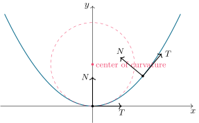
When $\kappa(s) \neq 0$ , the radius of curvature is $R(s) = 1/\abs{\kappa(s)}$ and the center of curvature is $\tilde\gamma(s) + \frac{1}{\kappa(s)} N(s)$ ; the circle with that center and radius $R(s)$ is the osculating circle, the best circular approximation of the curve at $\tilde\gamma(s)$ .

Example 18.15 (The osculating circle of the exponential)

For $y = \eu^x$ at the point $(0, 1)$ : $f'(0) = f''(0) = 1$ , so by the graph formula below,

\kappa(0) = \frac{1}{(1 + 1)^{3/2}} = \frac1{2\sqrt2}, \qquad R = 2\sqrt2 .

The unit tangent is $T = \frac{(1, 1)}{\sqrt2}$ , the direct normal $N = \frac{(-1, 1)}{\sqrt2}$ , and the center of curvature is

(0, 1) + 2\sqrt2\cdot\frac{(-1, 1)}{\sqrt2} = (-2,\ 3) :

the osculating circle has equation $(x + 2)^2 + (y - 3)^2 = 8$ . As a check of the “best circular approximation” claim: solving the circle’s equation for $y$ near $(0,1)$ and expanding gives $y = 1 + x + \frac{x^2}2 + O(x^3)$ — exactly the second-order Taylor expansion of $\eu^x$ . The osculating circle matches value, slope and second derivative; an ordinary tangent circle would match only the first two.

Example 18.16 (The evolute of a circle is its center)

For the circle of radius $R$ traversed counterclockwise, $\kappa = 1/R$ and $N$ points toward the center, so the center of curvature $\tilde\gamma + \frac1\kappa N$ is the center of the circle, for every $s$ : the osculating circle of a circle is the circle itself, and the locus of centers of curvature collapses to a point. This degenerate case calibrates Exercise 18.6: there the evolute’s velocity is $-\frac{\kappa'}{\kappa^2}N$ , which vanishes identically precisely when $\kappa$ is constant.

Proposition 18.17 (Curvature in an arbitrary parametrization)

For a regular $\mathcal{C}^2$ plane arc $\gamma(t) = (x(t), y(t))$ ,

\kappa(t) = \frac{x'(t)\,y''(t) - y'(t)\,x''(t)} {\bigl(x'(t)^2 + y'(t)^2\bigr)^{3/2}} ,

in particular $\kappa = \dfrac{y''}{(1 + y'^2)^{3/2}}$ for a graph $y = f(x)$ .

Proof. Write $v(t) = \norm{\gamma'(t)} = s'(t)$ , so $\gamma' = vT$ (composing the unit-speed data with $s$ ). Differentiating,

\gamma'' = v'T + v\,T'\cdot s' = v'T + v^2\kappa N .

Now take the determinant (in the canonical oriented basis) of $(\gamma', \gamma'')$ : since $\det(T, T) = 0$ and $\det(T, N) = 1$ ,

\det(\gamma', \gamma'') = \det(vT,\ v'T + v^2\kappa N) = v^3\kappa .

The left side is $x'y'' - y'x''$ , and $v^3 = (x'^2 + y'^2)^{3/2}$ . The graph case is the parametrization $t \mapsto (t, f(t))$ . ∎

Example 18.18 (Circle, line, parabola)

A line has $\kappa = 0$ (and conversely: $T' = 0$ means $T$ constant, so $\tilde\gamma(s) = \tilde\gamma(0) + sT$ , a line). The circle of radius $R$ traversed counterclockwise has $\kappa = 1/R$ : with $\gamma(t) = (R\cos t, R\sin t)$ , the formula gives $\kappa = R^2/R^3$ . For the parabola $y = x^2/2$ : $\kappa(x) = 1/(1 + x^2)^{3/2}$ , maximal at the vertex — the parabola is most sharply bent where it turns around.

Remark 18.19 (Common pitfalls around curvature)

(i) The algebraic curvature of a plane arc changes sign when the orientation of the arc or of the plane is reversed: only $\abs\kappa$ and $R = 1/\abs\kappa$ are purely geometric. A circle traversed clockwise has $\kappa = -1/R$ . (ii) The graph formula $\kappa = f''/(1 + f'^2)^{3/2}$ silently chooses the parametrization by $x$ ; applying it to a curve that is not a graph near the point (vertical tangent) is the classical blunder. (iii) At a point where $\gamma' = 0$ nothing is defined — neither $T$ nor $\kappa$ — and the trajectory may genuinely break (Example 18.5); always check regularity before differentiating the unit tangent. (iv) In space, $\kappa = \norm{T'} \geq 0$ by convention: there is no sign to get wrong, but also no sign to exploit — inflection-type information moves into the torsion. (v) Finally, $\kappa$ is a derivative with respect to arc length: for a non-unit-speed parametrization, forgetting the factor $v^3$ in Proposition 18.17 is the most frequent error in practice.

The parabola y = x2/2, its moving Frenet frame (T, N), and the osculating circle at the vertex (radius 1, since (0) = 1). The frame turns as the point moves; curvature is the rate of that turning per unit of arc length. — **Figure 18.1.** The parabola $y = x^2/2$ , its moving Frenet frame $(T, N)$ , and the osculating circle at the vertex (radius $1$ , since $\kappa(0) = 1$ ). The frame turns as the point moves; curvature is the rate of that turning per unit of arc length.

Theorem 18.20 (Curvature determines the curve)

Let $\kappa \colon J \to \R$ be continuous. There exists a unit-speed $\mathcal{C}^2$ arc in the plane with curvature $\kappa$ , and it is unique up to a direct isometry (rotation followed by translation).

Proof. Existence. Fix $s_0 \in J$ and set $\varphi(s) = \int_{s_0}^s \kappa(u)\,\dd u$ , then

\tilde\gamma(s) = \Bigl(\int_{s_0}^s \cos\varphi(u)\,\dd u,\ \int_{s_0}^s \sin\varphi(u)\,\dd u\Bigr).

Then $T(s) = (\cos\varphi(s), \sin\varphi(s))$ is a unit vector, $N(s) = (-\sin\varphi, \cos\varphi)$ , and

T'(s) = \varphi'(s)\,(-\sin\varphi, \cos\varphi) = \kappa(s)\,N(s) :

the arc is unit-speed with curvature $\kappa$ .

Uniqueness. Let $\gamma_1, \gamma_2$ be unit-speed arcs with the same curvature. Each unit tangent lifts to an angle function, by an explicit construction: view $T_j$ as the complex number $z_j = a_j + \iu b_j$ of modulus $1$ , pick $\varphi_j(0)$ with $z_j(0) = \eu^{\iu\varphi_j(0)}$ , and set

\varphi_j(s) = \varphi_j(0) + \int_0^s\det\bigl(T_j, T_j'\bigr)(u)\,\dd u .

From $\abs{z_j} = 1$ : $\operatorname{Re}(\conj{z_j}\,z_j') = 0$ , so $\conj{z_j}\,z_j' = \iu\det(T_j, T_j') = \iu\,\varphi_j'$ , i.e. $z_j' = \iu\varphi_j'z_j$ ; then

\bigl(z_j\,\eu^{-\iu\varphi_j}\bigr)' = \eu^{-\iu\varphi_j}\bigl(z_j' - \iu\varphi_j'z_j\bigr) = 0,

so $z_j = \eu^{\iu\varphi_j}$ throughout: $T_j = (\cos\varphi_j, \sin\varphi_j)$ with $\varphi_j$ of class $\mathcal C^1$ . Moreover $\det(T_j, T_j') = \det(T_j, \kappa N_j) = \kappa$ , so $\varphi_j' = \kappa$ . Hence $\varphi_2 = \varphi_1 + c$ for a constant $c$ : $T_2$ is $T_1$ rotated by the fixed angle $c$ , so integrating, $\gamma_2 = \rho(\gamma_1) + w$ where $\rho$ is the rotation of angle $c$ and $w$ a constant vector. ∎

Remark 18.21

This is the one-dimensional prototype of a fundamental theorem of geometry: a complete set of local invariants (here, one function) classifies the object up to rigid motion. The three-dimensional version below needs two invariants.

Example 18.22 (Constant curvature means circle)

Take $\kappa \equiv \kappa_0 > 0$ in the existence formula: $\varphi(s) = \kappa_0 s$ and

\tilde\gamma(s) = \Bigl(\frac{\sin\kappa_0s}{\kappa_0},\ \frac{1 - \cos\kappa_0s}{\kappa_0}\Bigr) :

the circle of radius $1/\kappa_0$ centered at $(0, 1/\kappa_0)$ , traversed at unit speed. By the uniqueness half of the theorem, every unit-speed arc of constant curvature $\kappa_0$ is a piece of a circle of radius $1/\kappa_0$ (or a line if $\kappa_0 = 0$ ) — the converse of the computation in Example 18.18, and the plane case of Exercise 18.9.

Example 18.23 (Reconstructing a curve from its curvature)

Which unit-speed curve has radius of curvature $R(s) = 1 + s^2$ ? Following the existence proof with $\kappa(s) = \frac1{1+s^2}$ and $s_0 = 0$ : $\varphi(s) = \arctan s$ , so

T(s) = (\cos\arctan s,\ \sin\arctan s) = \Bigl(\frac{1}{\sqrt{1+s^2}},\ \frac{s}{\sqrt{1+s^2}}\Bigr),

and integrating,

\tilde\gamma(s) = \Bigl(\ln\bigl(s + \sqrt{1 + s^2}\bigr),\ \sqrt{1 + s^2} - 1\Bigr).

Setting $x = \ln(s + \sqrt{1+s^2})$ , i.e. $s = \sinh x$ , the second coordinate is $\cosh x - 1$ : the curve is the catenary $y = \cosh x - 1$ . This closes the loop with Exercise 18.3, where we computed $R = \cosh^2 x = 1 + \sinh^2 x = 1 + s^2$ directly: the fundamental theorem guarantees the catenary is the only curve with this curvature profile, up to a direct isometry.

Remark 18.24 (Where curvature is used next)

The decomposition $\gamma'' = v'T + v^2\kappa N$ obtained in the proof of Proposition 18.17 is the kinematics of every curved motion: tangential versus centripetal acceleration. Curvature returns for surfaces (Chapter 19) through the curvature of curves drawn on them, and the envelope calculus of this chapter’s weekend problem — evolutes, caustics — is the geometric optics of wavefronts. The Year 3 volume takes the intrinsic point of view up again for submanifolds of $\R^n$ .

18.4 Frenet frame in space

Now let $\tilde\gamma \colon J \to \R^3$ be a unit-speed $\mathcal{C}^3$ arc that is biregular: $T'(s) \neq 0$ for all $s$ . Then $\kappa(s) = \norm{T'(s)} > 0$ defines the curvature (no sign in space: there is no preferred normal orientation), and we set:

N(s) = \frac{T'(s)}{\kappa(s)} \quad\text{(principal normal)}, \qquad B(s) = T(s) \wedge N(s) \quad\text{(binormal)} ,

so that $(T, N, B)$ is a direct orthonormal frame, the Frenet frame. The plane through $\tilde\gamma(s)$ spanned by $T, N$ is the osculating plane.

Theorem 18.25 (Frenet formulas in space)

There is a continuous function $\tau$ , the torsion, with

T' = \kappa N, \qquad N' = -\kappa T + \tau B, \qquad B' = -\tau N .

Proof. The first formula is the definition of $N$ . Each of the vectors $T, N, B$ has constant norm $1$ and they are pairwise orthogonal; differentiating the six relations $\langle X, Y\rangle = \delta_{XY}$ shows the matrix of $(T', N', B')$ in the basis $(T, N, B)$ is antisymmetric: indeed $\langle X', Y\rangle + \langle X, Y'\rangle = 0$ and $\langle X', X\rangle = 0$ . Its $(N, T)$ entry is $\langle N', T\rangle = -\langle N, T'\rangle = -\kappa$ , and its $(T, B)$ -column entry $\langle T', B\rangle = \kappa\langle N, B\rangle = 0$ . Naming the remaining free entry $\tau = \langle N', B\rangle$ gives exactly the three displayed formulas: antisymmetry fills in $\langle B', N\rangle = -\tau$ and $\langle B', T\rangle = 0$ . Continuity of $\tau = \langle N', B\rangle$ is clear since $N'$ and $B$ are continuous ( $\tilde\gamma$ is $\mathcal{C}^3$ , so $N = T'/\kappa$ is $\mathcal{C}^1$ ). ∎

Example 18.26 (The Darboux vector)

The three Frenet formulas compress into one. Set $\omega(s) = \tau\,T + \kappa\,B$ (the Darboux vector). Using $B \wedge T = N$ , $T \wedge N = B$ , $N \wedge B = T$ :

\omega \wedge T = \kappa\,N = T', \qquad \omega \wedge N = \tau\,B - \kappa\,T = N', \qquad \omega \wedge B = -\tau\,N = B' :

each frame vector evolves by $X' = \omega \wedge X$ , the kinematic signature of an instantaneous rotation with angular velocity vector $\omega$ . The frame spins at rate $\norm\omega = \sqrt{\kappa^2 + \tau^2}$ about the moving axis $\omega$ ; curvature is the component of the spin about the binormal, torsion the component about the tangent. For the helix, $\omega$ is a constant vector along the cylinder’s axis — which is exactly why the helix’s frame precesses evenly. The antisymmetry of the Frenet matrix, exploited in Exercise 18.7, is the matrix form of this single geometric fact.

Proposition 18.27 (Torsion measures planarity)

A biregular arc is contained in a plane if and only if $\tau \equiv 0$ ; in that case the plane is the (constant) osculating plane.

Proof. If $\tau \equiv 0$ , then $B' = 0$ , so $B$ is a constant unit vector $B_0$ , and

\frac{\dd}{\dd s}\langle \tilde\gamma(s), B_0\rangle = \langle T(s), B_0\rangle = 0 :

$\langle \tilde\gamma, B_0\rangle$ is constant, so the arc lies in a plane orthogonal to $B_0$ . Conversely, if the arc lies in a plane $P$ , then $T$ and $T'$ (hence $N$ ) are parallel to the direction of $P$ for all $s$ ; so $B = T \wedge N$ is one of the two unit normals of $P$ , and being continuous it is constant; then $0 = B' = -\tau N$ with $N \neq 0$ forces $\tau \equiv 0$ . ∎

Example 18.28 (A tilted circle has zero torsion)

The arc $\gamma(t) = \bigl(\cos t,\ \tfrac{\sin t}{\sqrt2},\ \tfrac{\sin t}{\sqrt2}\bigr)$ lies in the plane $y = z$ , and is the unit circle of that plane (check: $\norm{\gamma(t)} = 1$ and the plane’s orthonormal basis $(1,0,0)$ , $(0, \tfrac1{\sqrt2}, \tfrac1{\sqrt2})$ exhibits the standard parametrization). Without any Frenet computation, Proposition 18.27 predicts $\tau \equiv 0$ , and the fixed binormal must be the plane’s unit normal $\pm(0, \tfrac1{\sqrt2}, -\tfrac1{\sqrt2})$ . Torsion does not measure being “tilted in space”; it measures leaving a plane. Only the helix’s nonzero $b$ below produces genuine torsion.

Example 18.29 (The helix)

For the helix $\gamma(t) = (a\cos t, a\sin t, bt)$ , $a > 0$ , we computed $s = ct$ with $c = \sqrt{a^2 + b^2}$ . Then

T = \frac1c(-a\sin t,\ a\cos t,\ b), \qquad T' \cdot \frac{\dd t}{\dd s} = \frac{1}{c^2}(-a\cos t, -a\sin t, 0),

so $\kappa = a/c^2 = a/(a^2 + b^2)$ and $N = (-\cos t, -\sin t, 0)$ : the principal normal points horizontally toward the axis. Next $B = T \wedge N = \frac1c(b\sin t, -b\cos t, a)$ , and $B' \frac{\dd t}{\dd s} = \frac{b}{c^2}(\cos t, \sin t, 0) = -\tau N$ gives

\boxed{\ \kappa = \frac{a}{a^2 + b^2}, \qquad \tau = \frac{b}{a^2 + b^2}. \ }

Both invariants are constant — and one can show, conversely, that the only biregular curves with constant $\kappa > 0$ and constant $\tau$ are helices (circles when $\tau = 0$ ). Note the signs: $b > 0$ gives a right-handed helix with positive torsion.

Example 18.30 (Curvature and torsion without arc length; the twisted cubic)

Reparametrizing by arc length is usually impossible in closed form, so the invariants must be extracted from the raw derivatives. Write $v = \norm{\gamma'} = s'$ ; then $\gamma' = vT$ and, as in the proof of Proposition 18.17,

\gamma'' = v'T + v^2\kappa N, \qquad \gamma' \wedge \gamma'' = v^3\kappa\,(T \wedge N) = v^3\kappa\,B .

Taking norms ( $\kappa \geq 0$ in space):

\kappa = \frac{\norm{\gamma' \wedge \gamma''}}{v^3} .

Differentiating $\gamma''$ once more and converting $N' = v(-\kappa T + \tau B)$ (chain rule through $s$ ), the only $B$ -component comes from the last term:

\gamma''' = \bigl(v'' - v^3\kappa^2\bigr)T + \bigl(v'v\kappa + (v^2\kappa)'\bigr)N + v^3\kappa\tau\,B,

so that, pairing with $\gamma' \wedge \gamma'' = v^3\kappa B$ ,

\det(\gamma', \gamma'', \gamma''') = \langle\gamma' \wedge \gamma'',\ \gamma'''\rangle = v^6\kappa^2\tau, \qquad\text{i.e.}\qquad \tau = \frac{\det(\gamma', \gamma'', \gamma''')}{\norm{\gamma' \wedge \gamma''}^2} .

Application to the twisted cubic $\gamma(t) = (t,\ t^2,\ t^3)$ at $t = 0$ : $\gamma' = (1, 0, 0)$ , $\gamma'' = (0, 2, 0)$ , $\gamma''' = (0, 0, 6)$ , so $v = 1$ ,

\gamma' \wedge \gamma'' = (0, 0, 2), \qquad \kappa(0) = 2, \qquad \det(\gamma', \gamma'', \gamma''') = 12, \qquad \tau(0) = \frac{12}{4} = 3 .

Closing insight: both formulas are ratios in which the speed $v$ cancels to the exact degree needed — $\kappa$ scales like a second derivative per unit length, $\tau$ like the mixed volume of three derivatives per squared area — which is why they are geometric while $\gamma''$ itself is not.

Remark 18.31 (Fundamental theorem for space curves)

As in the plane, the pair $(\kappa, \tau)$ with $\kappa > 0$ determines a biregular arc up to direct isometry of $\R^3$ : the Frenet formulas form a linear differential system for the frame $(T, N, B)$ , to which the Cauchy–Lipschitz theory of Chapter 16 applies; orthonormality of the solution frame is preserved because the coefficient matrix is antisymmetric (same Gram-matrix argument as in Exercise 18.7), and the curve is recovered by integrating $T$ . We leave the details to the reader as a substantial but instructive exercise.

18.5 Local study: position with respect to the tangent

Proposition 18.32 (Local shape at a regular point)

Let $\gamma$ be a plane arc of class $\mathcal{C}^k$ at $t_0$ , with $p$ the smallest index with $\gamma^{(p)}(t_0) \neq 0$ and $q$ the smallest index $> p$ with $\gamma^{(q)}(t_0)$ not collinear with $\gamma^{(p)}(t_0)$ (assuming both exist, $q \leq k$ ). In the basis $(u, v) = (\gamma^{(p)}(t_0), \gamma^{(q)}(t_0))$ centered at $\gamma(t_0)$ , Taylor–Young gives coordinates

X(t) \sim \frac{(t - t_0)^p}{p!}, \qquad Y(t) \sim \frac{(t - t_0)^q}{q!} .

The local picture depends only on the parities of $p$ and $q$ :

$p$ odd, $q$ even	ordinary point	curve crosses no line, stays on one side of tangent
$p$ odd, $q$ odd	inflection point	curve crosses its tangent
$p$ even, $q$ odd	cusp of the first kind	both branches on opposite sides of tangent
$p$ even, $q$ even	cusp of the second kind	both branches on the same side

Proof. Taylor–Young at order $q$ (the function $\gamma$ is $\mathcal{C}^q$ near $t_0$ ):

\gamma(t) - \gamma(t_0) = \sum_{j=p}^{q} \frac{(t-t_0)^j}{j!}\,\gamma^{(j)}(t_0) + o\bigl((t-t_0)^q\bigr).

By the choice of $p$ and $q$ , each $\gamma^{(j)}(t_0)$ with $p \leq j < q$ is collinear with $u$ ; collecting components in the basis $(u, v)$ : $X(t) = \frac{(t-t_0)^p}{p!}(1 + o(1))$ and $Y(t) = \frac{(t-t_0)^q}{q!}(1 + o(1))$ . The sign table of $X$ and $Y$ for $t \gtrless t_0$ — governed exactly by the parities — gives the four pictures: for instance if $p$ is even, $X > 0$ on both sides (both branches leave in the direction $+u$ : a cusp), and the side of the tangent line ( $\operatorname{sign} Y$ ) flips with $q$ odd. ∎

Example 18.33

For $\gamma(t) = (t^2, t^3)$ at $t_0 = 0$ (Example 18.5): $\gamma'' (0)= (2, 0)$ , $\gamma'''(0) = (0, 6)$ , so $p = 2$ , $q = 3$ : a cusp of the first kind, the familiar picture of the semicubical parabola. For $\gamma(t) = (t, t^3)$ at $0$ : $p = 1$ , $q = 3$ : inflection — the cubic crosses its tangent.

Remark 18.34 (Perspectives within this volume)

Curves feed the next chapters in three ways. Drawn on a surface, they define its tangent planes and its first fundamental form (Chapter 19), and their lengths are computed by restricting the ambient metric — the chapter ahead is largely this chapter relativized. The envelope calculus of the weekend problem meets double integrals in Chapter 20, where the astroid’s area is recomputed by Green’s formula (Exercise 20.5) — one curve, two theories, matching answers. And the Frenet system already used the linear differential equations of Chapter 16 (existence, uniqueness, and the orthogonality-preservation argument of Exercise 18.7): the fundamental theorem of curves is a differential equations theorem wearing geometric clothes.

Remark 18.35 (Method: running the local study)

In practice the classification is a four-step routine. One, differentiate at $t_0$ until the first nonzero derivative appears: its index is $p$ , its value the vector $u$ . Two, keep differentiating until a derivative not collinear with $u$ appears: index $q$ , vector $v$ . Three, read the parities $(p, q)$ in the table. Four, draw: the curve leaves along $+u$ if $p$ is odd (along $u$ then back along $u$ if $p$ is even), on the side of $v$ dictated by the sign of $Y$ . Two cautions. The frame $(u, v)$ is generally not orthonormal — the table describes positions relative to the tangent line, not angles or distances, so do not read curvature off the picture. And intermediate derivatives collinear with $u$ are allowed between ranks $p$ and $q$ (they only shift the expansion of $X$ ); what must not happen is stopping at the first nonzero derivative and guessing $q = p + 1$ : for $\gamma(t) = (t^2, t^4 + t^5)$ the naive guess $q = 3$ is wrong, as $\gamma^{(3)}(0)$ is still collinear with $\gamma''(0)$ — this is precisely Exercise 18.5.

18.6 Exercises

Exercise 18.1 ★

Compute the length of one arch of the cycloid $\gamma(t) = (t - \sin t,\ 1 - \cos t)$ , $t \in [0, 2\pi]$ . (Use $1 - \cos t = 2\sin^2(t/2)$ .)

Solution

Solution of Exercise 18.1.

$\gamma'(t) = (1 - \cos t,\ \sin t)$ , so

\norm{\gamma'(t)}^2 = (1 - \cos t)^2 + \sin^2 t = 2 - 2\cos t = 4\sin^2\tfrac t2 ,

and $\norm{\gamma'(t)} = 2\sin\frac t2$ (nonnegative on $[0, 2\pi]$ ). Hence

L = \int_0^{2\pi} 2\sin\tfrac t2\,\dd t = \Bigl[-4\cos\tfrac t2\Bigr]_0^{2\pi} = 8 :

one arch of the cycloid has length $8$ (for a wheel of radius $1$ ) — a famous result of Wren, with no $\pi$ in sight.

Exercise 18.2 ★

Compute the curvature of the ellipse $\gamma(t) = (a\cos t,\ b\sin t)$ ( $a > b > 0$ ) and locate the points of maximal and minimal curvature.

Solution

Solution of Exercise 18.2.

With $x = a\cos t$ , $y = b\sin t$ : $x' = -a\sin t$ , $y' = b\cos t$ , $x'' = -a\cos t$ , $y'' = -b\sin t$ , so by Proposition 18.17

\kappa(t) = \frac{x'y'' - y'x''}{(x'^2 + y'^2)^{3/2}} = \frac{ab\sin^2 t + ab\cos^2 t} {(a^2\sin^2 t + b^2\cos^2 t)^{3/2}} = \frac{ab}{(a^2\sin^2 t + b^2\cos^2 t)^{3/2}} .

The denominator is minimal when $\sin t = 0$ (value $b^3$ , points $(\pm a, 0)$ ) and maximal when $\cos t = 0$ (value $a^3$ , points $(0, \pm b)$ ), since $a > b$ . Hence $\kappa$ is maximal at the ends of the major axis, $\kappa_{\max} = a/b^2$ , and minimal at the ends of the minor axis, $\kappa_{\min} = b/a^2$ : the ellipse bends most sharply at the tips of its long axis.

Exercise 18.3 ★

Show that the arc length of the graph of $f(x) = \cosh x$ over $[0, x]$ equals $\sinh x$ , and compute the curvature of this curve (the catenary). Verify that $R(x) = 1/\kappa(x) = \cosh^2 x$ .

Solution

Solution of Exercise 18.3.

For the graph $\gamma(x) = (x, \cosh x)$ : $\norm{\gamma'(x)} = \sqrt{1 + \sinh^2 x} = \cosh x$ , so the arc length from $0$ to $x$ is $\int_0^x \cosh u\,\dd u = \sinh x$ . Curvature of a graph (Proposition 18.17):

\kappa(x) = \frac{f''(x)}{(1 + f'(x)^2)^{3/2}} = \frac{\cosh x}{\cosh^3 x} = \frac{1}{\cosh^2 x} ,

so $R(x) = \cosh^2 x$ , as announced. Note the neat coincidence $R(x) = 1 + s(x)^2$ with $s = \sinh x$ the arc length: the catenary’s radius of curvature grows with the square of the arc length from the vertex.

Exercise 18.4 ★★

(Logarithmic spiral) Let $\gamma(t) = e^{t}(\cos t,\ \sin t)$ , $t \in \R$ . Show that the angle between $\gamma(t)$ and $\gamma'(t)$ is constant, compute the arc length of $\gamma$ on $(-\infty, 0]$ (finite!), and the curvature.

Solution

Solution of Exercise 18.4.

$\gamma'(t) = e^t(\cos t - \sin t,\ \sin t + \cos t)$ , so

\langle \gamma(t), \gamma'(t)\rangle = e^{2t} \bigl(\cos t(\cos t - \sin t) + \sin t(\sin t + \cos t)\bigr) = e^{2t},

while $\norm{\gamma(t)} = e^t$ and $\norm{\gamma'(t)} = e^t\sqrt 2$ . Hence

\cos\angle\bigl(\gamma, \gamma'\bigr) = \frac{e^{2t}}{e^t \cdot e^t\sqrt2} = \frac{1}{\sqrt2} :

the tangent always makes the angle $\pi/4$ with the radius — the equiangular property of the logarithmic spiral. Arc length on $(-\infty, 0]$ :

\int_{-\infty}^0 \norm{\gamma'(t)}\,\dd t = \sqrt2\int_{-\infty}^0 e^t\,\dd t = \sqrt 2 ,

finite although the spiral winds infinitely many times around the origin. Curvature: with $x'y'' - y'x''$ computed from $\gamma'' = e^t(-2\sin t,\ 2\cos t)$ ,

x'y'' - y'x'' = e^{2t}\bigl(2\cos t(\cos t - \sin t) + 2\sin t(\sin t + \cos t)\bigr) = 2e^{2t},

so $\kappa(t) = \dfrac{2e^{2t}}{(e^t\sqrt2)^3} = \dfrac{1}{e^t\sqrt2}$ : the curvature is $1/(\sqrt2\, \norm{\gamma})$ , decaying as the spiral grows.

Exercise 18.5 ★★

Determine $p$ , $q$ and the local shape (ordinary, inflection, cusp) of $\gamma(t) = (t^2,\ t^4 + t^5)$ at $t = 0$ , and of $\gamma(t) = (t^3,\ t^4)$ at $t = 0$ .

Solution

Solution of Exercise 18.5.

First arc: $\gamma(t) = (t^2,\ t^4 + t^5)$ . Derivatives at $0$ : $\gamma'' = (2, 0) \neq 0$ , so $p = 2$ . Then $\gamma^{(3)}(0) = (0, 0)$ , $\gamma^{(4)}(0) = (0, 24)$ , not collinear with $(2, 0)$ : $q = 4$ . Both even: cusp of the second kind — both branches leave in the direction $+u = (1,0)$ and stay on the same side of the tangent. (Indeed $y = x^2 \pm x^{5/2}$ on the two branches: same sign for small $x$ .)

Second arc: $\gamma(t) = (t^3, t^4)$ . $\gamma'(0) = \gamma''(0) = 0$ , $\gamma^{(3)}(0) = (6, 0)$ : $p = 3$ , odd. Next $\gamma^{(4)}(0) = (0, 24)$ : $q = 4$ , even. Odd–even: ordinary point — despite the vanishing velocity, the trajectory $y = x^{4/3}$ crosses the origin smoothly, staying above its tangent $y = 0$ .

Exercise 18.6 ★★

Let $\gamma$ be a unit-speed plane arc with $\kappa(s) > 0$ for all $s$ , and let $c(s) = \gamma(s) + \frac{1}{\kappa(s)}N(s)$ be the center of curvature (the curve $c$ is the evolute). Assuming $\kappa$ is $\mathcal{C}^1$ , show that $c'(s) = -\frac{\kappa'(s)}{\kappa(s)^2}N(s)$ : the evolute is tangent to the normal lines of $\gamma$ .

Solution

Solution of Exercise 18.6.

Differentiate $c(s) = \gamma(s) + \dfrac{1}{\kappa(s)}N(s)$ using the plane Frenet formulas (Theorem 18.13):

c'(s) = T(s) - \frac{\kappa'(s)}{\kappa(s)^2}N(s) + \frac{1}{\kappa(s)}\,\bigl(-\kappa(s)T(s)\bigr) = -\frac{\kappa'(s)}{\kappa(s)^2}\,N(s) ,

the tangent terms cancelling exactly. So the velocity of the evolute is carried by $N(s)$ , which directs the normal line of $\gamma$ at $\gamma(s)$ — and the point $c(s)$ lies on that very normal line: the evolute is the envelope of the normals. (Where $\kappa' = 0$ the evolute has a singular point; this is what produces the cusps of the evolute of an ellipse.)

Exercise 18.7 ★★★

Let $A(s)$ be a continuous family of antisymmetric $3 \times 3$ matrices and $F' = F A$ a matrix solution with $F(s_0)$ orthogonal. Show that $F(s)$ is orthogonal for all $s$ . (Differentiate $G = F F^{\mathsf T}$ and use uniqueness in Cauchy–Lipschitz.) Explain the relevance to the Frenet system.

Solution

Solution of Exercise 18.7.

Let $G(s) = F(s)F(s)^{\mathsf T}$ . Then, using $F' = FA$ and $(F^{\mathsf T})' = (F')^{\mathsf T} = A^{\mathsf T}F^{\mathsf T}$ ,

G' = F'F^{\mathsf T} + F(F^{\mathsf T})' = FAF^{\mathsf T} + FA^{\mathsf T}F^{\mathsf T} = F(A + A^{\mathsf T})F^{\mathsf T} = 0

by antisymmetry. So $G$ is constant on the interval, equal to $G(s_0) = F(s_0)F(s_0)^{\mathsf T} = I$ : $F(s)$ is orthogonal for every $s$ . (Alternatively, without computing $G'$ to zero: both $G$ and the constant $I$ solve the linear system $Y' = YA + A^{\mathsf T}Y$ with the same initial value, and Cauchy–Lipschitz uniqueness for linear systems, Chapter 16, forces $G \equiv I$ .)

Relevance: the Frenet system $(T, N, B)' = (T, N, B)\,A(s)$ has the antisymmetric coefficient matrix

A = \begin{pmatrix} 0 & -\kappa & 0\\ \kappa & 0 & -\tau\\ 0 & \tau & 0\end{pmatrix}

(columns expressing $T', N', B'$ ). The computation above shows that a solution frame that starts orthonormal stays orthonormal — the key step in the fundamental theorem reconstructing a curve from $(\kappa, \tau)$ .

Exercise 18.8 ★★★

(Total curvature of a closed convex curve) Let $\tilde\gamma$ be a unit-speed $\mathcal{C}^2$ closed plane arc of length $L$ (so $\tilde\gamma(s + L) = \tilde\gamma(s)$ ), traversed once counterclockwise. Using the angle function $\varphi$ with $T = (\cos\varphi, \sin\varphi)$ from Theorem 18.20, explain why $\varphi(L) - \varphi(0)$ is a multiple of $2\pi$ , and show that $\int_0^L \kappa(s)\,\dd s = \varphi(L) - \varphi(0)$ . (For a circle of radius $R$ : $\int \kappa = \frac1R \cdot 2\pi R = 2\pi$ . The theorem of turning tangents asserts the value $2\pi$ for every simple closed curve; you are not asked to prove that.)

Solution

Solution of Exercise 18.8.

By Theorem 18.20 (uniqueness part), there is a $\mathcal{C}^1$ angle function $\varphi$ with $T(s) = (\cos\varphi(s), \sin\varphi(s))$ and $\varphi' = \kappa$ . Hence

\int_0^L \kappa(s)\,\dd s = \varphi(L) - \varphi(0) .

Since the arc is closed of period $L$ , $T(L) = T(0)$ : $(\cos\varphi(L), \sin\varphi(L)) = (\cos\varphi(0), \sin\varphi(0))$ , so $\varphi(L) - \varphi(0) \in 2\pi\Z$ . The total curvature of a closed curve is therefore always an integer multiple of $2\pi$ — the integer being the winding number of the tangent (the number of full turns $T$ makes). For the circle of radius $R$ : $\kappa = 1/R$ and $L = 2\pi R$ , total curvature $2\pi$ , winding number $1$ ; the theorem of turning tangents states this value holds for every simple closed curve.

Exercise 18.9 ★★★

Show that a biregular space curve with constant $\kappa > 0$ and $\tau = 0$ is (an arc of) a circle of radius $1/\kappa$ . (Use Proposition 18.27, then show the center $\gamma + \frac1\kappa N$ is constant.)

Solution

Solution of Exercise 18.9.

Since $\tau \equiv 0$ , the curve lies in a plane (Proposition 18.27); work in that plane. Consider the candidate center

c(s) = \gamma(s) + \frac{1}{\kappa}N(s) \qquad (\kappa \text{ constant}).

Differentiating with the Frenet formulas ( $N' = -\kappa T + \tau B = -\kappa T$ here):

c'(s) = T + \frac1\kappa(-\kappa T) = 0 ,

so $c$ is a constant point $\Omega$ . Then $\norm{\gamma(s) - \Omega} = \norm{-\frac1\kappa N(s)} = \frac1\kappa$ for all $s$ : the curve lies on the circle of center $\Omega$ and radius $1/\kappa$ (in its plane), and being a nonconstant arc of it, it is an arc of that circle.

Exercise 18.10 ★

Compute the arc length of the parabola $y = x^2/2$ over $\intcc0a$ and show that it equals

\tfrac12\Bigl(a\sqrt{1 + a^2} + \ln\bigl(a + \sqrt{1 + a^2}\bigr)\Bigr).

Solution

Solution of Exercise 18.10.

For the graph $\gamma(x) = (x, x^2/2)$ , $\norm{\gamma'(x)} = \sqrt{1 + x^2}$ , so $L = \int_0^a\sqrt{1+x^2}\,\dd x$ . Substituting $x = \sinh u$ ( $\dd x = \cosh u\,\dd u$ , $u$ from $0$ to $u_a = \ln(a + \sqrt{1+a^2})$ ):

L = \int_0^{u_a}\cosh^2 u\,\dd u = \frac12\bigl[u + \sinh u\cosh u\bigr]_0^{u_a} = \frac12\Bigl(\ln\bigl(a + \sqrt{1+a^2}\bigr) + a\sqrt{1+a^2}\Bigr),

using $\cosh^2 u = \frac{1 + \cosh 2u}2$ and $\sinh u_a = a$ , $\cosh u_a = \sqrt{1 + a^2}$ .

Exercise 18.11 ★★

Let $\gamma$ be a regular $\mathcal C^2$ arc in $\R^n$ all of whose tangent lines pass through a fixed point $P$ . Prove that the trajectory of $\gamma$ is contained in a straight line. (Parametrize by arc length, write $\gamma(s) + \lambda(s)T(s) = P$ and differentiate.)

Solution

Solution of Exercise 18.11.

Parametrize by arc length (Theorem 18.9) and set $\lambda(s) = \langle P - \gamma(s), T(s)\rangle$ , a $\mathcal C^1$ function; since $P$ lies on the tangent line at $\gamma(s)$ , the vector $P - \gamma(s)$ is collinear with $T(s)$ , so $P = \gamma(s) + \lambda(s)T(s)$ . Differentiating,

0 = T(s) + \lambda'(s)T(s) + \lambda(s)T'(s) = \bigl(1 + \lambda'(s)\bigr)T(s) + \lambda(s)T'(s),

and $T'(s) \perp T(s)$ (differentiate $\norm T^2 = 1$ ), so both components vanish: $\lambda' = -1$ and $\lambda T' = 0$ . Then $\lambda(s) = c - s$ vanishes at most once, so $T' = 0$ on a dense set, hence everywhere by continuity: $T$ is a constant unit vector and $\gamma(s) = \gamma(s_0) + (s - s_0)T$ : a straight line (through $P$ , as it must be).

Exercise 18.12 ★★★

(Fundamental theorem for space curves) Let $\kappa > 0$ and $\tau$ be continuous functions on an interval $J$ . Carry out the program of the remark following Example 18.29: (a) show that the linear system $F' = FA(s)$ , with $A(s)$ the antisymmetric Frenet matrix built from $\kappa, \tau$ and $F(s_0)$ a direct orthonormal frame, has a unique global solution, which remains a direct orthonormal frame; (b) construct a unit-speed biregular curve with curvature $\kappa$ and torsion $\tau$ ; (c) prove uniqueness up to a direct isometry of $\R^3$ .

Solution

Solution of Exercise 18.12.

(a) The Frenet matrix

A(s) = \begin{pmatrix} 0 & -\kappa & 0\\ \kappa & 0 & -\tau\\ 0 & \tau & 0\end{pmatrix}

has continuous entries, so the linear system $F' = FA(s)$ , $F(s_0) = F_0$ (a direct orthonormal matrix) has a unique solution on all of $J$ (Theorem 16.4). By Exercise 18.7, $F(s)$ is orthogonal for every $s$ ; $\det F$ is continuous with values in $\{\pm1\}$ and equals $1$ at $s_0$ , so $F(s)$ is direct for all $s$ .

(b) Read off the rows $T, N, B$ of $F$ (so that $T' = \kappa N$ , $N' = -\kappa T + \tau B$ , $B' = -\tau N$ ) and set $\gamma(s) = \gamma_0 + \int_{s_0}^s T(u)\,\dd u$ . Then $\gamma' = T$ is a unit vector: unit speed; $T' = \kappa N$ with $\kappa > 0$ and $N$ unit orthogonal to $T$ , so $\gamma$ is biregular with curvature $\norm{T'} = \kappa$ and principal normal $N$ ; the binormal is $T \wedge N = B$ (direct orthonormal frame), and $B' = -\tau N$ identifies the torsion as $\tau$ .

(c) Let $\gamma_1, \gamma_2$ be unit-speed biregular curves with the same $(\kappa, \tau)$ . There is a unique direct isometry $\Phi = \rho + w$ ( $\rho \in SO(3)$ ) sending $\gamma_1(s_0)$ to $\gamma_2(s_0)$ and the Frenet frame of $\gamma_1$ at $s_0$ to that of $\gamma_2$ at $s_0$ . The curve $\Phi\circ\gamma_1$ is unit-speed with the same invariants (its frame is $\rho$ applied to that of $\gamma_1$ , and $\rho$ preserves cross products, being direct). Now the frames of $\Phi\circ\gamma_1$ and $\gamma_2$ both solve $F' = FA(s)$ with the same initial value, so they coincide by uniqueness; in particular the tangents agree, and integrating from the common point $s_0$ : $\Phi\circ\gamma_1 = \gamma_2$ .

18.7 Problem: envelopes — the astroid, two evolutes, and a caustic

A ladder of length 1 sliding down a wall (blue positions) never crosses the astroid x2/3 + y2/3 = 1 (red): the astroid is the envelope of the family of segments, tangent to every one of them. — A ladder of length $1$ sliding down a wall (blue positions) never crosses the astroid $x^{2/3} + y^{2/3} = 1$ (red): the astroid is the *envelope* of the family of segments, tangent to every one of them.

Problem 18.1

Weekend problem — the envelope machine and four classical curves

A one-parameter family of lines usually fails to cover the plane evenly: the lines pile up along a curve tangent to all of them, their envelope. Light rays make envelopes visible as caustics — the bright cusped curve in a mug of coffee. This problem builds the general envelope machine, then runs it four times: the sliding ladder (astroid), the normals of the parabola and of the cycloid (evolutes, with Huygens’ pendulum at the end), and the coffee-cup caustic (nephroid). Throughout, $D_t$ denotes the line of equation $a(t)\,x + b(t)\,y = c(t)$ , where $a, b, c$ are $\mathcal C^2$ functions with $(a(t), b(t)) \neq (0,0)$ , and $\Delta(t) = a(t)b'(t) - a'(t)b(t)$ .

Part I — The envelope machine.

Suppose $\Delta(t) \neq 0$ . Show that the characteristic system

$\begin{cases} a(t)\,x + b(t)\,y = c(t)\\ a'(t)\,x + b'(t)\,y = c'(t)\end{cases}$

has a unique solution $E(t) = (x(t), y(t))$ , given by $x = \dfrac{cb' - c'b}{\Delta}$ , $y = \dfrac{ac' - a'c}{\Delta}$ .
Assume moreover that $E$ is $\mathcal C^1$ near $t$ with $E'(t) \neq 0$ . Differentiating the first equation of the system, show $a(t)\,x'(t) + b(t)\,y'(t) = 0$ , and conclude that the curve $E$ passes through a point of $D_t$ with the direction of $D_t$ : the family is tangent to $E$ , which is called its envelope.
Sanity check: the tangent lines of the parabola $y = x^2/2$ at the points $(t, t^2/2)$ are $tx - y = t^2/2$ . Verify that the envelope machine returns the parabola itself.
(Envelope of the normals) Let $\gamma$ be unit-speed with $\kappa(s) \neq 0$ . The normal line at $\gamma(s)$ is $\{M : \langle M - \gamma(s), T(s) \rangle = 0\}$ . Show that its characteristic system forces $\langle M - \gamma(s), N(s)\rangle = 1/\kappa(s)$ , hence that the characteristic point is the center of curvature: the envelope of the normals is the evolute, recovering Exercise 18.6. Check $\Delta(s) = \kappa(s)$ .
Two degenerations. For the pencil $D_\theta : x\cos \theta + y\sin\theta = 0$ , show that the characteristic point is the origin for every $\theta$ (the “envelope” collapses to a point, and $E' = 0$ : question 2 does not apply). For a family of parallel lines ( $a, b$ constant), show $\Delta \equiv 0$ and that the characteristic system is in general inconsistent: no envelope.

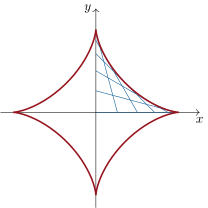
Part II — The sliding ladder and the astroid. A segment of length $1$ slides with one end $P_t = (\cos t, 0)$ on the floor and the other $Q_t = (0, \sin t)$ on the wall, $t \in \intoo0{\pi/2}$ .

Show that the line $(P_tQ_t)$ has equation $x\sin t + y\cos t = \sin t\cos t$ , and that the envelope machine gives the characteristic point

$E(t) = (\cos^3 t,\ \sin^3 t) :$

the astroid, of implicit equation $x^{2/3} + y^{2/3} = 1$ (extended to the other quadrants by symmetry).
Show that $E'(0) = 0$ and, using the local classification (Proposition 18.32), that the astroid has a cusp of the first kind at $(1, 0)$ — and likewise at its four axis points.
Compute $\norm{E'(t)} = \tfrac32\abs{\sin 2t}$ and deduce that the total length of the astroid is $6$ .
Where does the ladder touch the astroid? Show $E(t) = P_t + \sin^2 t\,(Q_t - P_t)$ : the contact point divides the ladder in the ratio $\sin^2 t : \cos^2 t$ , sweeping it from one end to the other as the ladder slides.
Compute the area enclosed by the astroid: show that the first-quadrant area is $3\int_0^{\pi/2}\sin^4 t\cos^2 t\,\dd t$ , evaluate the integral by linearization ( $\sin^2 2t = \tfrac{1 - \cos 4t}2$ ), and conclude that the total area is $3\pi/8$ .

Part III — The evolute of the parabola. Let $\gamma(t) = (t, t^2/2)$ .

Show that the normal line at $\gamma(t)$ has equation $x + t\,y = t + t^3/2$ .
Run the envelope machine: show that the envelope of the normals is

$E(t) = \Bigl(-t^3,\ 1 + \tfrac32 t^2\Bigr),$

with implicit equation $x^2 = \tfrac8{27}(y - 1)^3$ : a semicubical parabola.
Cross-check with question 4: compute the center of curvature $\gamma(t) + \frac1{\kappa(t)}N(t)$ from $\kappa(t) = (1 + t^2)^{-3/2}$ (Example 18.18) and recover the same point.
Show that the evolute has a cusp of the first kind at $(0, 1)$ , the center of curvature at the vertex — the point where $\kappa$ is extremal, as predicted by the formula $c' = -\frac{\kappa'}{\kappa^2}N$ of Exercise 18.6.
How many normals of the parabola pass through a given point $(x_0, y_0)$ ? Show the answer is governed by the cubic $\tfrac{t^3}2 + (1 - y_0)\,t - x_0 = 0$ ; treat the axis case $x_0 = 0$ completely (one normal for $y_0 < 1$ , three for $y_0 > 1$ ), and interpret the evolute as the transition curve.

Part IV — The coffee-cup caustic. Parallel rays of direction $(1, 0)$ strike the inside of the mirror circle $x^2 + y^2 = 1$ ; the ray hitting $P_\theta = (\cos\theta, \sin\theta)$ reflects according to the law of reflection.

From the mirror symmetry in the normal (the radius), justify that the reflected direction is $v = u - 2\langle u, n\rangle n$ with $u = (1,0)$ , $n = (\cos\theta, \sin\theta)$ , and compute $v = -(\cos2\theta, \sin2\theta)$ .
Show that the reflected ray lies on the line

$x\sin 2\theta - y\cos 2\theta = \sin\theta .$
Run the envelope machine ( $\Delta = 2$ ): show that the caustic is

$E(\theta) = \Bigl(\tfrac{3\cos\theta - \cos3\theta}4,\ \tfrac{3\sin\theta - \sin3\theta}4\Bigr),$

the nephroid.
Compute $E'(\theta) = \tfrac32\sin\theta\, (\cos2\theta, \sin2\theta)$ ; check that the tangent direction is the reflected-ray direction (question 16), locate the two cusps $(\pm\tfrac12, 0)$ , and show that the reflected ray crosses the axis $y = 0$ at $x = \frac1{2\cos\theta}$ — so nearly axial rays focus at $x = \tfrac12$ : the focal length $R/2$ of a mirror of radius $R$ .
Show that the nephroid has total length $6$ and that near $\theta = 0$ ,

$E(\theta) - \bigl(\tfrac12, 0\bigr) = \bigl(\tfrac34\theta^2 + o(\theta^2),\ \theta^3 + o(\theta^3)\bigr) :$

a cusp of the first kind, pointing along the axis.
Explain in one paragraph why the caustic is bright: through every point just outside the caustic pass two reflected rays, through every point on it the rays are “infinitely concentrated” (the map $(\theta, \text{distance along ray}) \mapsto \R^2$ has a critical point exactly on the envelope).

Part V — Huygens: the cycloid is its own evolute. Let $\gamma(t) = (t - \sin t,\ 1 - \cos t)$ , $t \in \intoo0{2\pi}$ , one arch of the cycloid.

Compute $\kappa(t) = -\dfrac1{4\sin(t/2)}$ and the center of curvature; show that the evolute is

$c(t) = (t + \sin t,\ \cos t - 1),$

and that the substitution $t = u + \pi$ exhibits it as the original cycloid translated by $(\pi, -2)$ : the evolute of a cycloid is a congruent cycloid (Huygens).
Verify that the radius of curvature at the apex $t = \pi$ equals $4$ , which is half the length $8$ of one arch (Exercise 18.1); locate the cusp of the evolute directly below the apex, at distance $4$ .
(The string property) Let $\gamma$ be unit-speed with $\kappa > 0$ , $\kappa$ of class $\mathcal C^1$ and $R = 1/\kappa$ strictly monotone. Using $c' = R'N$ , show that the arc length of the evolute between $c(s_0)$ and $c(s_1)$ is $\abs{R(s_1) - R(s_0)}$ . Interpret: a taut string unwound from the evolute, of length $R(s_0)$ at the start, has its free end trace the original curve — so a pendulum swinging between two cycloidal cheeks of Huygens’ clock describes a cycloid.
Synthesis. The machine of Part I produced the astroid, a semicubical parabola, a nephroid and a cycloid. For each of the four families, state in one sentence where the hypotheses $\Delta \neq 0$ and $E' \neq 0$ held or failed, and what geometric event (cusp, focus, degeneracy) each failure of $E' \neq 0$ signalled. Where must extrema of curvature appear on the envelope of the normals, and why?

Solution

Solution of Problem 18.1.

1. The system is linear in $(x, y)$ with determinant $\Delta(t) = a b' - a'b \neq 0$ : Cramer’s rule gives the unique solution

x = \frac{c b' - c' b}{\Delta}, \qquad y = \frac{a c' - a' c}{\Delta}.

2. Since $a(t)x(t) + b(t)y(t) = c(t)$ identically, differentiating gives $a'x + b'y + ax' + by' = c'$ ; the second characteristic equation kills $a'x + b'y - c'$ , so $a(t)x'(t) + b(t)y'(t) = 0$ : $E'(t)$ is orthogonal to $(a, b)$ , hence parallel to $(-b, a)$ , the direction of $D_t$ . As $E(t) \in D_t$ (first equation) and $E'(t) \neq 0$ , the line $D_t$ is exactly the tangent line of the curve $E$ at $E(t)$ .

3. Here $(a, b, c) = (t, -1, t^2/2)$ , so $\Delta = t\cdot0 - 1\cdot(-1) = 1$ and

x = \frac{c b' - c' b}{\Delta} = \tfrac{t^2}2\cdot 0 + t = t, \qquad y = \frac{a c' - a' c}{\Delta} = t\cdot t - \tfrac{t^2}2 = \tfrac{t^2}2 :

the envelope of the tangent lines of the parabola is the parabola, as it should be.

4. The normal line is $\langle M, T(s)\rangle = \langle\gamma(s), T(s)\rangle$ : coefficients $a = T_1$ , $b = T_2$ , $c = \langle\gamma, T\rangle$ . Differentiating with Frenet ( $T' = \kappa N$ ): $a' = \kappa N_1$ , $b' = \kappa N_2$ , and $c' = \langle T, T\rangle + \langle\gamma, \kappa N\rangle = 1 + \kappa\langle\gamma, N\rangle$ . The second characteristic equation $\kappa\langle M, N\rangle = 1 + \kappa\langle\gamma, N\rangle$ reads $\kappa\langle M - \gamma, N\rangle = 1$ . The first says $M - \gamma \perp T$ , so $M - \gamma = \mu N$ with $\mu = 1/\kappa$ : the characteristic point is $\gamma + \frac1\kappa N$ , the center of curvature, and the envelope of the normals is the evolute of Exercise 18.6. Finally $\Delta = T_1\kappa N_2 - \kappa N_1 T_2 = \kappa\det(T, N) = \kappa \neq 0$ .

5. Pencil: the system $x\cos\theta + y\sin\theta = 0$ , $-x\sin\theta + y\cos\theta = 0$ has determinant $1$ and solution $(0,0)$ for every $\theta$ : $E \equiv (0,0)$ , $E' \equiv 0$ , and there is no curve — merely the common point of all the lines. Parallel family: $a' = b' = 0$ gives $\Delta \equiv 0$ and the second equation $0 = c'(t)$ , which fails as soon as the family actually moves: no characteristic point, and indeed a family of parallel lines touches no curve along all its members.

6. The line through $(\cos t, 0)$ and $(0, \sin t)$ is $\frac x{\cos t} + \frac y{\sin t} = 1$ , i.e. $x\sin t + y\cos t = \sin t\cos t$ . With $(a, b, c) = (\sin t, \cos t, \sin t\cos t)$ : $a' = \cos t$ , $b' = -\sin t$ , $c' = \cos 2t$ , $\Delta = -\sin^2 t - \cos^2 t = -1$ . Cramer:

\begin{align*} x &= \frac{cb' - c'b}{-1} = \sin^2 t\cos t + \cos 2t\cos t = \cos t\,(\sin^2 t + \cos^2 t - \sin^2 t) = \cos^3 t,\\ y &= \frac{ac' - a'c}{-1} = \sin t\cos^2 t - \sin t\cos 2t = \sin t\,(\cos^2 t - \cos^2 t + \sin^2 t) = \sin^3 t . \end{align*}

And $(\cos^3t)^{2/3} + (\sin^3t)^{2/3} = 1$ : the astroid.

7. $E'(t) = 3(-\cos^2 t\sin t,\ \sin^2 t\cos t)$ vanishes at $t = 0$ . There, $E''(0) = (-3, 0) \neq 0$ gives $p = 2$ ; the $x$ -component of $E$ is even in $t$ , so $E'''(0) = (0, 6)$ , not collinear: $q = 3$ . Even–odd: cusp of the first kind at $(1, 0)$ (Proposition 18.32), with tangent along the $x$ -axis. The symmetries $x \mapsto -x$ , $y \mapsto -y$ , $(x, y) \mapsto (y, x)$ of the astroid transport the cusp to $(-1, 0)$ and $(0, \pm1)$ .

8. $E'(t) = 3\sin t\cos t\,(-\cos t, \sin t)$ , so $\norm{E'(t)} = 3\abs{\sin t\cos t} = \tfrac32\abs{\sin 2t}$ . One quadrant: $\int_0^{\pi/2}\tfrac32\sin 2t\,\dd t = \tfrac32$ , and by symmetry the total length is $4 \cdot \tfrac32 = 6$ .

9. $E(t) - P_t = (\cos^3 t - \cos t,\ \sin^3 t) = \sin^2 t\,(-\cos t,\ \sin t) = \sin^2 t\,(Q_t - P_t)$ . So the contact point is the barycenter of $(P_t, \cos^2 t)$ and $(Q_t, \sin^2 t)$ : as $t$ runs from $0$ to $\pi/2$ it slides from the floor end to the wall end of the ladder.

10. In the first quadrant the region under the astroid has area $\int_0^1 y\,\dd x$ with $x = \cos^3 t$ decreasing from $1$ to $0$ as $t$ goes from $0$ to $\pi/2$ :

\int_0^1 y\,\dd x = \int_{\pi/2}^{0}\sin^3 t\,(-3\cos^2 t\sin t)\,\dd t = 3\int_0^{\pi/2}\sin^4 t\cos^2 t\,\dd t .

Linearize: $\sin^4 t\cos^2 t = (\sin t\cos t)^2\sin^2 t = \tfrac18\bigl(\sin^2 2t - \sin^2 2t\cos 2t\bigr)$ , and $\int_0^{\pi/2}\sin^2 2t\,\dd t = \tfrac\pi4$ while $\int_0^{\pi/2}\sin^2 2t\cos 2t\,\dd t = \bigl[\tfrac{\sin^3 2t}6\bigr]_0^{\pi/2} = 0$ . So the integral is $\tfrac\pi{32}$ , the quadrant area $\tfrac{3\pi}{32}$ , and the enclosed area $4 \cdot \tfrac{3\pi}{32} = \tfrac{3\pi}8$ .

11. The tangent at $\gamma(t) = (t, t^2/2)$ is directed by $(1, t)$ , so the normal line is $\{(x, y) : (x - t) + t\,(y - t^2/2) = 0\}$ , i.e. $x + t\,y = t + \tfrac{t^3}2$ .

12. $(a, b, c) = (1, t, t + t^3/2)$ : $a' = 0$ , $b' = 1$ , $c' = 1 + \tfrac32 t^2$ , $\Delta = 1$ . Then $y = ac' - a'c = 1 + \tfrac32t^2$ and

x = cb' - c'b = t + \tfrac{t^3}2 - t\Bigl(1 + \tfrac32t^2\Bigr) = -t^3 .

Eliminating $t$ : $t^2 = \tfrac23(y - 1)$ and $x^2 = t^6 = \tfrac8{27}(y - 1)^3$ : a semicubical parabola with vertex $(0, 1)$ .

13. $T = (1, t)/\sqrt{1+t^2}$ , $N = (-t, 1)/\sqrt{1+t^2}$ , and $\kappa = (1+t^2)^{-3/2}$ , so

\gamma + \frac1\kappa N = (t, \tfrac{t^2}2) + (1+t^2)\,(-t, 1) = \Bigl(-t^3,\ 1 + \tfrac32t^2\Bigr),

the same curve: the envelope of the normals is the locus of the centers of curvature, as question 4 promised.

14. $E'(t) = (-3t^2, 3t)$ vanishes at $t = 0$ ; $E''(0) = (0, 3) \neq 0$ gives $p = 2$ and $E'''(0) = (-6, 0)$ gives $q = 3$ : a cusp of the first kind at $(0, 1)$ . The vertex is where $\kappa = (1+t^2)^{-3/2}$ is maximal, so $\kappa'(0) = 0$ and the evolute’s velocity $-\frac{\kappa'}{\kappa^2}N$ vanishes exactly there: cusps of the evolute sit at the extrema of curvature.

15. The normal at parameter $t$ passes through $(x_0, y_0)$ iff $x_0 + t\,y_0 = t + \tfrac{t^3}2$ , i.e.

\frac{t^3}2 + (1 - y_0)\,t - x_0 = 0 ,

a cubic in $t$ : one or three real roots (counted without multiplicity, for generic points). On the axis $x_0 = 0$ it factors as $t\bigl(\tfrac{t^2}2 + 1 - y_0\bigr) = 0$ : the root $t = 0$ (the axis is the normal at the vertex), plus $t = \pm\sqrt{2(y_0 - 1)}$ when $y_0 > 1$ . So: one normal for $y_0 < 1$ , three for $y_0 > 1$ , and at $y_0 = 1$ the triple root marks the cusp of the evolute. In general a double root of the cubic means the point satisfies both the line equation and its $t$ -derivative — it lies on the envelope: the evolute is precisely the boundary between the one-normal and three-normal regions.

16. Reflection in the mirror reverses the normal component of the direction and keeps the tangential one: writing $u = \langle u, n\rangle n + u_{\mathrm{tan}}$ , the reflected direction is $u_{\mathrm{tan}} - \langle u, n\rangle n = u - 2\langle u, n\rangle n$ . Here $\langle u, n\rangle = \cos\theta$ , so

v = (1, 0) - 2\cos\theta\,(\cos\theta, \sin\theta) = (1 - 2\cos^2\theta,\ -2\sin\theta\cos\theta) = -(\cos2\theta,\ \sin2\theta).

17. The reflected ray passes through $P_\theta = (\cos\theta, \sin\theta)$ with direction $(\cos2\theta, \sin2\theta)$ ; a normal vector is $(-\sin2\theta, \cos2\theta)$ , so the line is

-\sin2\theta\,(x - \cos\theta) + \cos2\theta\,(y - \sin\theta) = 0,

and the constant is $-\sin2\theta\cos\theta + \cos2\theta\sin\theta = -\sin\theta$ : multiplying by $-1$ , $x\sin2\theta - y\cos2\theta = \sin\theta$ .

18. $(a, b, c) = (\sin2\theta, -\cos2\theta, \sin\theta)$ : $a' = 2\cos2\theta$ , $b' = 2\sin2\theta$ , $c' = \cos\theta$ , $\Delta = 2\sin^22\theta + 2\cos^22\theta = 2$ . Cramer, then product-to-sum formulas:

\begin{align*} x &= \frac{2\sin\theta\sin2\theta + \cos\theta\cos2\theta}{2} = \frac{(\cos\theta - \cos3\theta) + \frac12(\cos\theta + \cos3\theta)}{2} = \frac{3\cos\theta - \cos3\theta}4,\\ y &= \frac{\sin2\theta\cos\theta - 2\cos2\theta\sin\theta}2 = \frac{\frac12(\sin3\theta + \sin\theta) - (\sin3\theta - \sin\theta)}2 = \frac{3\sin\theta - \sin3\theta}4 : \end{align*}

the nephroid, a closed curve with two cusps.

19. Differentiating and factoring with $\sin3\theta - \sin\theta = 2\cos2\theta\sin\theta$ , $\cos\theta - \cos3\theta = 2\sin2\theta\sin\theta$ :

E'(\theta) = \tfrac34\bigl(\sin3\theta - \sin\theta,\ \cos\theta - \cos3\theta\bigr) = \tfrac32\sin\theta\,(\cos2\theta, \sin2\theta),

parallel to the reflected direction of question 16: each reflected ray is tangent to the caustic, as the envelope property demands. $E' = 0$ exactly at $\sin\theta = 0$ : $E(0) = (\tfrac12, 0)$ and $E(\pi) = (-\tfrac12, 0)$ , the two cusps. Setting $y = 0$ in the line equation: $x\sin2\theta = \sin\theta$ , so $x = \frac1{2\cos\theta} \to \frac12$ as $\theta \to 0$ : paraxial rays focus at distance $R/2$ from the center — the focal length of the spherical mirror.

20. $\norm{E'(\theta)} = \tfrac32\abs{\sin\theta}$ , so the length is $\tfrac32\int_0^{2\pi}\abs{\sin\theta}\, \dd\theta = \tfrac32\cdot4 = 6$ . Near $\theta = 0$ , with $\cos k\theta = 1 - \tfrac{k^2\theta^2}2 + O(\theta^4)$ and $\sin k\theta = k\theta - \tfrac{k^3\theta^3}6 + O(\theta^5)$ :

x - \tfrac12 = \frac{3\theta^2 + O(\theta^4)}{4} = \tfrac34\theta^2 + O(\theta^4), \qquad y = \frac{4\theta^3 + O(\theta^5)}{4} = \theta^3 + O(\theta^5) :

$p = 2$ , $q = 3$ , a cusp of the first kind pointing along the axis — the bright point of the coffee-cup caustic.

21. Parametrize the illuminated points by $\Phi(\theta, r) = P_\theta + r\,v_\theta$ (position along each reflected ray). The Jacobian determinant $\det(\partial_\theta\Phi, \partial_r\Phi) = \det(P_\theta' + rv_\theta', v_\theta)$ is affine in $r$ and vanishes for exactly one $r = r_*(\theta)$ — and $\Phi(\theta, r_*(\theta))$ is the characteristic point, since there the ray direction and the variation of the family become dependent. Off the envelope the map is a local diffeomorphism, and a point just inside the caustic is hit by two nearby rays (two solutions $\theta$ ), a point outside by none from that part of the family; on the caustic the two merge. Light intensity is inversely proportional to the Jacobian’s absolute value, so it blows up along the envelope: the caustic is the bright curve, brightest of all at the cusp, where the degeneracy is worst.

22. $x' = 1 - \cos t$ , $y' = \sin t$ , $x'' = \sin t$ , $y'' = \cos t$ , so $x'y'' - y'x'' = \cos t - 1$ and $\norm{\gamma'}^2 = 2(1 - \cos t) = 4\sin^2\tfrac t2$ ; by Proposition 18.17,

\kappa(t) = \frac{-(1 - \cos t)}{8\sin^3\tfrac t2} = \frac{-2\sin^2\tfrac t2}{8\sin^3\tfrac t2} = -\frac1{4\sin\tfrac t2} \qquad (0 < t < 2\pi).

With $T = (\sin\tfrac t2, \cos\tfrac t2)$ (divide $\gamma'$ by $2\sin\tfrac t2$ ) and $N = (-\cos\tfrac t2, \sin\tfrac t2)$ :

\gamma + \frac1\kappa N = \gamma - 4\sin\tfrac t2\,\Bigl(-\cos\tfrac t2,\ \sin\tfrac t2\Bigr) = \bigl(t - \sin t + 2\sin t,\ 1 - \cos t - 2(1 - \cos t)\bigr),

i.e. $c(t) = (t + \sin t,\ \cos t - 1)$ . Substituting $t = u + \pi$ :

c = \bigl(u + \pi - \sin u,\ -\cos u - 1\bigr) = \bigl((u - \sin u) + \pi,\ (1 - \cos u) - 2\bigr) :

the cycloid $\gamma(u)$ translated by $(\pi, -2)$ . The evolute of a cycloid is a congruent cycloid, hanging one level below.

23. $R(t) = 1/\abs{\kappa(t)} = 4\sin\tfrac t2$ , so $R(\pi) = 4$ : half of the arch length $8$ computed in Exercise 18.1. The evolute’s velocity $c'(t) = (1 + \cos t, -\sin t)$ vanishes at $t = \pi$ : the cusp is $c(\pi) = (\pi, -2)$ , directly below the apex $\gamma(\pi) = (\pi, 2)$ , at distance $4 = R(\pi)$ , exactly the length of the osculating radius there.

24. From Exercise 18.6, $c'(s) = -\frac{\kappa'(s)}{\kappa(s)^2}N(s) = R'(s)\,N(s)$ , so $\norm{c'(s)} = \abs{R'(s)}$ and, for monotone $R$ ,

\int_{s_0}^{s_1}\norm{c'(s)}\,\dd s = \Bigl|\int_{s_0}^{s_1}R'(s)\,\dd s\Bigr| = \abs{R(s_1) - R(s_0)} .

Say $R$ decreases. A string laid along the evolute beyond $c(s_0)$ and prolonged by the segment from $c(s_0)$ to $\gamma(s_0)$ (which is tangent to the evolute, by question 4) has, when peeled off up to $c(s)$ and stretched taut, straight part of length $R(s_0) - \bigl(R(s_0) - R(s)\bigr) = R(s)$ pointing from $c(s)$ along the normal — landing exactly on $\gamma(s)$ : the free end traces the original curve (“involute”). Huygens hung a pendulum between two cycloidal cheeks: the cord wraps on the evolute, so the bob describes a cycloid — the tautochrone, whose oscillation period does not depend on the amplitude.

25. Tangents of the parabola: $\Delta = 1$ and $E' = (1, t) \neq 0$ everywhere — smooth envelope (the parabola itself). Sliding ladder: $\Delta = -1$ , but $E' = \tfrac32\sin 2t\,(-\cos t, \sin t)$ vanishes at the quadrant ends — the four cusps of the astroid. Normals of the parabola and of the cycloid: $\Delta = \kappa \neq 0$ , and $E' = R'N$ vanishes exactly where the curvature is extremal — cusps of the evolutes at $(0,1)$ and $(\pi, -2)$ . Caustic: $\Delta = 2$ , and $E' = \tfrac32\sin\theta\,(\cos2\theta, \sin2\theta)$ vanishes at $\theta = 0, \pi$ — the two cusps of the nephroid, the focal points of the mirror. Extrema of curvature must produce cusps on the envelope of the normals, since the evolute’s velocity is $R'N$ : this is why the evolute of the ellipse has four cusps (four vertices), and the degenerate families (pencil, parallels) are the cases where the machine outputs a point or nothing at all.