University Mathematics — Year 2 · Bachelor Year 2

23Probability Generating Functions

The power series of Chapter 11 return with a probabilistic mission: to an $\N$ -valued random variable we attach the power series with coefficients $\P(X = n)$ . This generating function converts sums of independent variables into products, moments into derivatives at $1$ , and hard combinatorial identities into one-line multiplications. The chapter closes the book with two showpieces: the Poisson approximation of rare events, and the extinction criterion for branching processes — a genuinely infinite probabilistic computation solved entirely by the geometry of a convex curve.

23.1 Definition and basic properties

Definition 23.1 (Probability generating function)

Let $X$ be an $\N$ -valued random variable, $p_n = \P(X = n)$ . The probability generating function of $X$ is the sum of the power series

G_X(t) = \E\bigl(t^X\bigr) = \sum_{n=0}^{\infty} p_n\,t^n .

Example 23.2 (First reflexes)

A constant variable $X = c$ has $G_X(t) = t^c$ ; a shift obeys $G_{X+c}(t) = t^c\,G_X(t)$ ; and evaluating at special points reads off information without any expansion: $G_X(0) = \P(X = 0)$ , $G_X(1) = 1$ , and $G_X(-1) = \P(X\text{ even}) - \P(X\text{ odd})$ , the parity balance exploited in Exercise 23.10. These one-liners are used silently everywhere below — and the evaluation $G_X(0)$ is exactly how extinction probabilities will be extracted from iterated generating functions at the end of the chapter.

Proposition 23.3 (Radius and first properties)

The series defining $G_X$ has radius of convergence $\geq 1$ ; $G_X$ is defined and continuous on $\intcc{-1}{1}$ , $\mathcal{C}^\infty$ on $\intoo{-1}{1}$ , with $G_X(1) = 1$ and $\abs{G_X(t)} \leq 1$ there. Moreover $G_X$ determines the law of $X$ :

p_n = \frac{G_X^{(n)}(0)}{n!} .

Proof. Since $\sum p_n = 1$ converges, the terms $p_n\,1^n$ are bounded, so the radius is $\geq 1$ (Abel’s lemma, Chapter 11); at $t = \pm1$ the series converges absolutely ( $\sum p_n = 1$ dominates); better, on the whole interval $\intcc{-1}1$ ,

\sup_{\abs t\leq1}\,\abs{p_nt^n} = p_n \quad\text{with}\quad \sum_np_n < \infty :

the series converges normally on $\intcc{-1}1$ , so its sum is continuous there (Theorems 10.16 and 10.4). Smoothness inside and the coefficient formula are the general theory of power series; the coefficients being recoverable, two variables with the same generating function have the same law. ∎

Example 23.4 (The classical laws)

Bernoulli $\mathcal{B}(p)$ : $G(t) = 1 - p + pt$ .
Binomial $\mathcal{B}(n, p)$ : $G(t) = \sum_k \binom nk (pt)^k(1-p)^{n-k} = (1 - p + pt)^n$ (binomial theorem).
Geometric $\mathcal{G}(p)$ : $G(t) = \sum_{k\geq1}(1-p)^{k-1}p\,t^k = \dfrac{pt}{1 - (1-p)t}$ (radius $\frac{1}{1-p} > 1$ ).
Poisson $\mathcal{P}(\lambda)$ : $G(t) = \sum_k e^{-\lambda}\frac{(\lambda t)^k}{k!} = e^{\lambda(t - 1)}$ (radius $\infty$ ).

Example 23.5 (Integrating the generating function)

Derivatives of $G_X$ at $1$ give positive moments; the integral gives a negative one. From $\int_0^1t^k\dd t = \frac1{k+1}$ and term-by-term integration (normal convergence on $\intcc01$ ):

\int_0^1G_X(t)\,\dd t = \sum_{k\geq0}\frac{\P(X = k)}{k+1} = \E\Bigl(\frac1{1+X}\Bigr).

For $X \sim \mathcal P(\lambda)$ :

\E\Bigl(\frac1{1+X}\Bigr) = \int_0^1\eu^{\lambda(t-1)}\,\dd t = \frac{1 - \eu^{-\lambda}}{\lambda},

recovering in one line the series computation of Example 22.10. The generating function is a two-way instrument: differentiate at $1$ for the moments $\E(X)$ , $\E(X(X-1))$ , integrate over $\intcc01$ for $\E\bigl(\frac1{1+X}\bigr)$ — one analytic object, queried in whichever direction the problem needs.

Example 23.6 (A law with radius exactly one)

Let $\P(X = k) = \dfrac{6}{\pi^2k^2}$ for $k \geq 1$ — a probability law by Basel’s identity (Example 14.12). Its generating function $G(t) = \frac6{\pi^2}\sum_{k\geq1}\frac{t^k}{k^2}$ has radius of convergence exactly $1$ : the general bound “radius $\geq 1$ ” of Proposition 23.3 cannot be improved. And the mean is

\sum_{k\geq1}k\,\P(X = k) = \frac6{\pi^2}\sum_{k\geq1}\frac1k = \infty :

$G$ is continuous on $\intcc{-1}1$ , smooth inside, but its derivative blows up at $1^-$ — the graph arrives at the point $(1, 1)$ with a vertical tangent. Heavy tails are visible geometrically on the generating function, at the single point $t = 1$ ; the moments theorem below makes this correspondence exact.

Theorem 23.7 (Moments from the generating function)

$X$ has an expectation if and only if $G_X$ is differentiable at $1^-$ (left derivative, finite), and then $\E(X) = G_X'(1)$ . Similarly $X$ has a second moment iff $G_X$ is twice differentiable at $1^-$ , and then

\E\bigl(X(X - 1)\bigr) = G_X''(1), \qquad V(X) = G_X''(1) + G_X'(1) - G_X'(1)^2 .

Proof. For $t \in \intoo{0}{1}$ , term-by-term differentiation inside the disk gives $G_X'(t) = \sum_{n\geq1} np_n t^{n-1}$ , a series with nonnegative coefficients: $t \mapsto G_X'(t)$ is nondecreasing on $\intoo{0}{1}$ , and by monotone convergence of partial sums (or Abel’s theorem for nonnegative coefficients, Chapter 11),

\lim_{t \to 1^-} G_X'(t) = \sum_{n\geq1} n\,p_n \in \intcc{0}{+\infty} ,

each side finite exactly when the other is. When finite, the mean value theorem squeezes the difference quotients $\frac{G_X(1) - G_X(t)}{1 - t}$ between values of $G_X'$ , so $G_X$ is differentiable at $1^-$ with $G_X'(1) = \sum np_n = \E(X)$ (by transfer). The second-order statement repeats the argument one level up: $G''_X(t) = \sum_{n\geq2}n(n-1)p_nt^{n-2}$ is nondecreasing on $\intoo01$ with monotone limit $\sum_nn(n-1)p_n = \E(X(X-1))$ , finite exactly when $X$ has a second moment. The variance formula then follows from König–Huygens:

V(X) = \E(X^2) - \E(X)^2 = \E\bigl(X(X-1)\bigr) + \E(X) - \E(X)^2 = G''_X(1) + G'_X(1) - G'_X(1)^2 .

∎

Example 23.8

Poisson: $G'(t) = \lambda e^{\lambda(t-1)}$ , so $\E(X) = \lambda$ ; $G''(1) = \lambda^2$ , so $V(X) = \lambda^2 + \lambda - \lambda^2 = \lambda$ — the computations of Chapter 22 in one line each.

Example 23.9 (The mode of a Poisson law)

Where is $\P(X = k)$ largest for $X \sim \mathcal P(\lambda)$ ? Consecutive weights compare through the ratio

\frac{\P(X = k+1)}{\P(X = k)} = \frac{\lambda}{k + 1} ,

which exceeds $1$ while $k < \lambda - 1$ and drops below $1$ once $k > \lambda - 1$ : the weights rise then fall, with mode $\floor\lambda$ (and a tie between $\lambda - 1$ and $\lambda$ when $\lambda$ is an integer: for $\lambda = 3$ , $\P(X = 2) = \P(X = 3) = \frac92\eu^{-3} \approx 0.224$ ). Ratio tests on the coefficients are often the fastest route to qualitative facts about a discrete law — no generating function needed, but the coefficients are the generating function, read term by term.

23.2 Sums of independent variables

Theorem 23.10 (Multiplicativity)

If $X$ and $Y$ are independent $\N$ -valued random variables, then

G_{X + Y}(t) = G_X(t)\,G_Y(t) \qquad (\abs t \leq 1),

and by induction $G_{X_1 + \dots + X_n} = \prod_i G_{X_i}$ for independent $X_1, \dots, X_n$ .

Proof. Two proofs, both instructive. Via expectations: $t^X$ and $t^Y$ are independent bounded variables, so (Theorem 22.11)

G_{X+Y}(t) = \E\bigl(t^{X+Y}\bigr) = \E\bigl(t^X t^Y\bigr) = \E\bigl(t^X\bigr)\E\bigl(t^Y\bigr) .

Via Cauchy products: the law of $X + Y$ is the convolution $\P(X + Y = n) = \sum_{k=0}^n \P(X = k)\P(Y = n - k)$ , and the Cauchy product theorem for absolutely convergent series (Chapter 7) multiplies the two power series exactly along this convolution. ∎

Example 23.11 (Stability of the classical laws)

Independent binomials with the same $p$ add: $(1 - p + pt)^m(1 - p + pt)^n = (1 - p + pt)^{m+n}$ , so $\mathcal{B}(m, p) + \mathcal{B}(n, p) = \mathcal{B}(m + n, p)$ — in particular a sum of $n$ independent Bernoulli variables is binomial, re-proving the law of the number of successes. Independent Poissons add: $e^{\lambda(t-1)}e^{\mu(t-1)} = e^{(\lambda + \mu)(t-1)}$ , so $\mathcal{P}(\lambda) + \mathcal{P}(\mu) = \mathcal{P}(\lambda + \mu)$ — the convolution computation of Exercise 22.2, now without computation.

Example 23.12 (Two dice, one polynomial squared)

For one fair die, $G(t) = \frac{t + t^2 + \dots + t^6}{6}$ ; for the sum of two,

G(t)^2 = \frac{1}{36}\bigl(t^2 + 2t^3 + 3t^4 + 4t^5 + 5t^6 + 6t^7 + 5t^8 + 4t^9 + 3t^{10} + 2t^{11} + t^{12}\bigr) :

the triangular law of dice sums ( $7$ is the mode, with probability $\frac6{36} = \frac16$ ), read off a polynomial square that one multiplies out once in a lifetime. The convolution formula would have required eleven separate counting arguments; the generating function does them all simultaneously, because multiplying polynomials is convolving coefficients. This mechanical translation — laws to coefficients, sums to products — is the whole business model of the chapter, and Exercise 23.11 pushes it to the surprising Sicherman dice.

Example 23.13 (Three dice and a coefficient extraction)

For the sum $S$ of three fair dice, $\P(S = 10)$ is the coefficient of $t^{10}$ in $\bigl(\frac{t + \dots + t^6}6\bigr)^3$ . Factor and expand with the binomial and geometric series:

\Bigl(\frac{t(1 - t^6)}{6(1 - t)}\Bigr)^{\!3} = \frac{t^3}{216}\,\bigl(1 - 3t^6 + 3t^{12} - t^{18}\bigr)\sum_{j\geq0}\binom{j+2}2t^j .

The coefficient of $t^{10}$ requires $t^7$ from the product: $j = 7$ with the term $1$ , and $j = 1$ with the term $-3t^6$ :

\P(S = 10) = \frac{1}{216}\Bigl(\binom92 - 3\binom32\Bigr) = \frac{36 - 9}{216} = \frac{27}{216} = \frac18 .

Direct enumeration of the $27$ triples is error-prone; the algebra is mechanical and scales to any number of dice — the inclusion–exclusion visible in $(1 - t^6)^3$ is doing the case analysis automatically.

Example 23.14 (Reading a law off its generating function)

Which law has $G(t) = \dfrac1{2 - t}$ ? Expand into a power series:

\frac{1}{2 - t} = \frac12\cdot\frac1{1 - t/2} = \sum_{k\geq0}\frac{t^k}{2^{k+1}} :

nonnegative coefficients summing to $G(1) = 1$ , so this is a genuine law, $\P(X = k) = 2^{-(k+1)}$ on $\N$ — a geometric law starting at $0$ . By uniqueness (Proposition 23.3), no other law shares this $G$ . Recognizing laws from their generating functions is a skill worth drilling: it is how the critical branching iterate $G_n(t) = \frac{n - (n-1)t}{n+1 - nt}$ of the weekend problem is unmasked as a geometric law conditioned on survival.

Remark 23.15

Stability goes one way only: sums of independent Poissons are Poisson, but differences are not — $X - Y$ takes negative values, so it has no generating function at all, and its law (the Skellam distribution) lies outside this chapter’s toolkit. Likewise $\mathcal B(m, p) + \mathcal B(n, p')$ with $p \neq p'$ is not binomial: the product $(1 - p + pt)^m(1 - p' + p't)^n$ has two distinct root locations, while every binomial pgf has a single repeated root. Reading stability off root patterns is a small preview of how much structure the polynomial encodes.

Remark 23.16 (The roots-of-unity filter)

Evaluating at $-1$ separates even from odd; evaluating at all $m$ -th roots of unity separates every residue class: with $\omega = \eu^{2\iu\pi/m}$ ,

\P(X \equiv r \bmod m) = \frac1m\sum_{j=0}^{m-1}\omega^{-jr}\,G_X(\omega^j),

since averaging $\omega^{j(k-r)}$ over $j$ yields $1$ if $k \equiv r$ and $0$ otherwise. Sample dividend: for the sum $S$ of two fair dice, each $G(\omega^j) = \frac16\sum_{k=1}^6 \omega^{jk} = -\frac16$ for $j \neq 0$ (the seven seventh roots of unity sum to zero), so

\P(7 \mid S) = \frac17\Bigl(1 + 6\cdot\frac1{36}\Bigr) = \frac16 ,

confirming the count from Example 23.12 — and the method scales to questions where direct counting does not.

Theorem 23.17 (Random sums: Wald’s identity for generating functions)

Let $(X_k)_{k\geq1}$ be independent $\N$ -valued variables with the same law and generating function $G_X$ , and let $N$ be an $\N$ -valued variable independent of the $X_k$ , with generating function $G_N$ . Then the random sum $S = X_1 + \dots + X_N$ (with $S = 0$ when $N = 0$ ) has generating function

G_S = G_N \circ G_X .

In particular, if $N$ and $X_1$ have expectations, $\E(S) = \E(N)\,\E(X_1)$ .

Proof. Condition on $N$ (total probability, Theorem 21.14): for $\abs t \leq 1$ ,

G_S(t) = \sum_{n=0}^\infty \P(N = n)\, \E\bigl(t^{X_1 + \dots + X_n}\bigr) = \sum_{n=0}^\infty \P(N = n)\,G_X(t)^n = G_N\bigl(G_X(t)\bigr),

using multiplicativity for each fixed $n$ and the summability of the whole double family ( $\abs{G_X(t)} \leq 1$ ). The exchange of summations is Fubini for summable families (Chapter 7). Differentiating at $1^-$ by the chain rule and Theorem 23.7: $\E(S) = G_N'(G_X(1))\,G_X'(1) = G_N'(1)G_X'(1) = \E(N)\E(X_1)$ . ∎

Example 23.18 (Compound Poisson: yearly insurance losses)

An insurer receives $N \sim \mathcal P(\lambda)$ claims in a year, each claim costing $X_k$ (integer units, i.i.d., pgf $G_X$ , mean $\mu$ , independent of $N$ ). By Theorem 23.17, the total loss $S$ has

G_S(t) = \eu^{\lambda(G_X(t) - 1)}, \qquad \E(S) = \lambda\mu ,

and differentiating twice at $1^-$ :

V(S) = \lambda\,G_X''(1) + \lambda^2\mu^2 + \lambda\mu - (\lambda\mu)^2 = \lambda\,\E(X^2) .

The variance involves the second moment of a single claim, not its variance: a compound Poisson sum feels the occasional large claim twice — once through how many, once through how big. For $\lambda = 10$ claims of geometric law with mean $2$ ( $\E X^2 = 6$ ): $\E S = 20$ , $V(S) = 60$ , and Chebyshev (Chapter 22) already yields usable solvency margins. This “randomly stopped sum” pattern is the same one that will drive the branching recursion of Proposition 23.23: composition of generating functions is the algebra of random populations.

Remark 23.19

The independence of $N$ from the summands is not decorative. Take $X_k \in \{0, 2\}$ with equal probabilities and let $N = X_1$ (flagrantly dependent): then $S = X_1 + \dots + X_N$ is $0$ when $X_1 = 0$ , and $2 + X_2$ when $X_1 = 2$ , so $\E(S) = \frac12(2 + 1) = \frac32$ , while $\E(N)\E(X_1) = 1\cdot1 = 1$ : Wald’s identity fails. When the number of terms is allowed to react to the terms themselves, the clean product structure collapses — the full theory of such “stopping” rules is the martingale chapter of the Year 3 volume.

23.3 Poisson approximation

Theorem 23.20 (Law of rare events)

Let $X_n \sim \mathcal{B}(n, p_n)$ with $n\,p_n \to \lambda > 0$ . Then for every $k \in \N$ :

\P(X_n = k) \xrightarrow[n\to\infty]{} e^{-\lambda}\frac{\lambda^k}{k!} :

the binomial law of many rare independent events converges to the Poisson law of parameter $\lambda$ .

Proof. Direct computation with $p_n = \frac{\lambda_n}{n}$ , $\lambda_n \to \lambda$ :

\P(X_n = k) = \binom nk p_n^k(1 - p_n)^{n-k} = \frac{n(n-1)\cdots(n-k+1)}{n^k}\cdot \frac{\lambda_n^k}{k!}\, \bigl(1 - \tfrac{\lambda_n}{n}\bigr)^{n-k} .

As $n \to \infty$ with $k$ fixed: the first factor tends to $1$ (product of $k$ factors $\to 1$ ); $\lambda_n^k \to \lambda^k$ ; and $\bigl(1 - \frac{\lambda_n}{n}\bigr)^{n-k} = \exp\bigl((n-k)\ln(1 - \frac{\lambda_n}{n})\bigr) \to e^{-\lambda}$ since $(n - k)\ln\bigl(1 - \frac{\lambda_n}{n}\bigr) \sim -\lambda_n \to -\lambda$ (Chapter 6). Alternatively, at the level of generating functions: $G_{X_n}(t) = \bigl(1 + \frac{\lambda_n(t-1)}{n}\bigr)^n \to e^{\lambda(t - 1)} = G_{\mathcal{P}(\lambda)}(t)$ for each fixed $t \in [0, 1]$ — convergence of generating functions, which (for $\N$ -valued variables) is equivalent to convergence of each $\P(X_n = k)$ ; see Exercise 23.9. ∎

Remark 23.21

This is why Poisson laws model counts of rare events — typos per page, radioactive decays per second, accidents per day at a crossing: each opportunity is nearly negligible, opportunities are many, and only the mean rate $\lambda$ survives in the limit.

Example 23.22 (Watching the Poisson limit converge)

Fix $\lambda = 2$ and let $X_n \sim \mathcal B(n, 2/n)$ . The no-event probability is exactly $\P(X_n = 0) = (1 - 2/n)^n$ :

n = 10:\ 0.107, \qquad n = 20:\ 0.122, \qquad n = 50:\ 0.130, \qquad n = 100:\ 0.133,

against the limit $\eu^{-2} \approx 0.135$ . The convergence is monotone and of speed $O(1/n)$ — expanding, $(1 - 2/n)^n = \eu^{-2}\bigl(1 - \tfrac2n + O(n^{-2})\bigr)$ — so for $n$ in the hundreds the Poisson model is already accurate to the third digit. This is the practical content of the law of rare events: the modeller never knows $n$ and $p$ separately (how many micro-opportunities for a typo does a page hold?), but only their product $\lambda$ , and the limit law mercifully depends on nothing else.

23.4 Branching processes

Consider a population starting from one ancestor; each individual, independently, has a random number of children with law $(p_k)_{k \in \N}$ and generating function $G$ (the offspring distribution). Let $Z_n$ be the size of generation $n$ ( $Z_0 = 1$ ), and let $m = G'(1) = \E(Z_1)$ be the mean offspring number.

Proposition 23.23

The generating function of $Z_n$ is the $n$ -th iterate $G_{Z_n} = G \circ G \circ \dots \circ G$ ( $n$ times), and the extinction probabilities $q_n = \P(Z_n = 0)$ satisfy

q_0 = 0, \qquad q_{n+1} = G(q_n),

and increase to the probability $q$ of eventual extinction, which is a fixed point of $G$ .

Proof. Generation $n + 1$ is the random sum of the offspring of the $Z_n$ members of generation $n$ , with counts independent of each other and of $Z_n$ : Theorem 23.17 gives $G_{Z_{n+1}} = G_{Z_n} \circ G$ , and induction from $G_{Z_0}(t) = t$ yields the $n$ -fold iterate — which, by associativity of composition, can equally be read as $G_{Z_{n+1}} = G \circ G_{Z_n}$ . Evaluating this second form at $0$ : $q_{n+1} = G_{Z_{n+1}}(0) = G\bigl(G_{Z_n}(0)\bigr) = G(q_n)$ . The events $\{Z_n = 0\}$ increase (extinct populations stay extinct), so $q_n \uparrow q = \P\bigl(\bigcup_n\{Z_n = 0\}\bigr)$ by monotone continuity (Theorem 21.6), and continuity of $G$ on $[0, 1]$ turns $q_{n+1} = G(q_n)$ into $q = G(q)$ at the limit. ∎

Example 23.24 (Watching extinction converge)

For the offspring law $(p_0, p_1, p_2) = (\tfrac14, \tfrac14, \tfrac12)$ of Example 23.27, $G(t) = \tfrac14 + \tfrac14t + \tfrac12t^2$ and the iteration $q_{n+1} = G(q_n)$ gives

q_1 = 0.25, \quad q_2 = 0.34375, \quad q_3 \approx 0.39502, \quad q_4 \approx 0.42678, \quad q_5 \approx 0.44776,

climbing toward the extinction probability $q = \tfrac12$ . The gaps $q - q_n$ are $0.25$ , $0.156$ , $0.105$ , $0.073$ , $0.052$ : each is roughly $\tfrac34$ of the previous, and indeed the mean value theorem gives $q - q_{n+1} = G'(c_n)(q - q_n)$ with $G'(q) = \tfrac14 + q = \tfrac34$ . Two morals: a family line still alive at generation $n$ has, built into the same computation, probability $q - q_n$ of being doomed later; and the convergence rate of the staircase in the figure below is the derivative at the fixed point — the weekend problem turns both observations into theorems.

Theorem 23.25 (Extinction criterion)

Assume $p_1 \neq 1$ . The extinction probability $q$ is the smallest fixed point of $G$ in $\intcc{0}{1}$ , and:

if $m \leq 1$ (subcritical or critical), $q = 1$ : extinction is certain;
if $m > 1$ (supercritical), $q < 1$ : the population survives forever with positive probability $1 - q$ .

Proof. $G$ is convex on $\intcc{0}{1}$ (power series with nonnegative coefficients: $G'' \geq 0$ ), nondecreasing, with $G(1) = 1$ .

Smallest fixed point: let $r \in \intcc{0}{1}$ be any fixed point. Then $q_0 = 0 \leq r$ , and inductively $q_{n+1} = G(q_n) \leq G(r) = r$ (monotonicity): so $q = \lim q_n \leq r$ .

Case $m \leq 1$ : suppose $r < 1$ is a fixed point. By the mean value theorem on $[r, 1]$ , there is $c \in \intoo{r}{1}$ with $G'(c) = \frac{G(1) - G(r)}{1 - r} = \frac{1 - r}{1 - r} = 1$ . But $G'$ is nondecreasing (convexity) with $\lim_{t\to1^-}G'(t) = m \leq 1$ , so $G' \leq 1$ on $\intoo{0}{1}$ ; the equality $G'(c) = 1$ then forces $G'$ to be constant equal to $1$ on $\intco{c}{1}$ , hence $G'' = \sum n(n-1)p_nt^{n-2} \equiv 0$ there. A power series with nonnegative coefficients vanishing on an interval has all these coefficients zero: $p_n = 0$ for $n \geq 2$ , so $G(t) = p_0 + p_1t$ and $1 = G'(c) = p_1$ — contradicting the hypothesis $p_1 \neq 1$ . So $1$ is the only fixed point: $q = 1$ .

Case $m > 1$ : near $1$ , $G(t) - t$ has derivative $G'(t) - 1 \to m - 1 > 0$ as $t \to 1^-$ , so $G(t) - t < G(1) - 1 = 0$ on some interval $\intoo{1 - \delta}{1}$ : the continuous function $G(t) - t$ is $\geq 0$ at $t = 0$ ( $G(0) = p_0 \geq 0$ ) and $< 0$ just below $1$ , so it vanishes at some $r < 1$ (intermediate value theorem). The smallest fixed point is then $q \leq r < 1$ . ∎

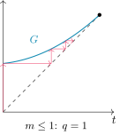
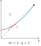
Extinction probabilities as a fixed-point iteration q_n+1 = G(q_n) starting at q_0 = 0 (red staircase). Left: a subcritical offspring law — the convex curve stays above the diagonal, the iteration climbs to the unique fixed point 1. Right: a supercritical law — the curve crosses the diagonal at q < 1, where the iteration stops: survival has probability 1 - q > 0. — **Figure 23.1.** Extinction probabilities as a fixed-point iteration $q_{n+1} = G(q_n)$ starting at $q_0 = 0$ (red staircase). Left: a subcritical offspring law — the convex curve stays above the diagonal, the iteration climbs to the unique fixed point $1$ . Right: a supercritical law — the curve crosses the diagonal at $q < 1$ , where the iteration stops: survival has probability $1 - q > 0$ .

Remark 23.26 (How to read the cobweb)

In the figure, a vertical move applies $G$ (from $(q_n, q_n)$ up to $(q_n, G(q_n))$ ), a horizontal move to the diagonal converts output into input: the staircase is the recursion $q_{n+1} = G(q_n)$ . Convexity of $G$ and $G(1) = 1$ leave only two geometries. Either the curve stays above the diagonal on $\intco01$ (mean $m \leq 1$ ): the staircase has nowhere to stop before $1$ . Or the curve crosses at some $q < 1$ ( $m > 1$ ): the staircase is trapped below the crossing and converges to it, at the geometric rate $G'(q) < 1$ quantified in Example 23.24. All the analysis of the extinction theorem is visible in this one picture — which is why it is worth drawing before computing.

Example 23.27

Offspring law: no child, one child, two children with probabilities $\frac14, \frac14, \frac12$ . Then $m = \frac14 + 1 = \frac54 > 1$ and $G(t) = \frac14 + \frac14 t + \frac12 t^2$ . Fixed points: $\frac12 t^2 - \frac34 t + \frac14 = 0$ , i.e. $2t^2 - 3t + 1 = (2t - 1)(t - 1) = 0$ : $q = \frac12$ . The family line dies out with probability $\frac12$ — and with probability $\frac12$ it lives forever.

Remark 23.28 (Perspectives within this volume)

The chapter is the book’s crossroads, and each ingredient arrived from a named place: the series algebra from Chapter 7 and Chapter 11, the probability from Chapter 21 (monotone continuity proves $q_n \uparrow q$ ) and Chapter 22 ( $G_X = \E(t^X)$ is an expectation, multiplicativity is the product theorem), the convexity from Chapter 8 through Chapter 17. Even the heavy-tail pathologies connect: the St Petersburg variable of the previous chapter has $G(t) = \sum_k2^{-k}t^{2^k}$ , a perfectly convergent series on $\intcc01$ whose derivative at $1^-$ diverges — infinite mean, visible at a glance. One object, every tool of the year: a fitting last chapter.

Remark 23.29 (Common pitfalls)

(i) Generating functions apply to $\N$ -valued variables only: for signed or non-integer variables the object $\E(t^X)$ loses its power-series structure (Year 3 replaces it with transforms adapted to $\R$ ). (ii) The first sanity check of any computed $G$ is $G(1) = 1$ ; the second is that the coefficients are nonnegative — a negative coefficient means an algebra slip, not a new law. (iii) In random sums, the composition order matters: $G_S = G_N \circ G_X$ , the outer function counting the terms; composing the other way is meaningless ( $G_X \circ G_N$ would count items of items). (iv) Multiplicativity needs independence and distinct sources of randomness: $G_{2X}(t) = G_X(t^2)$ , not $G_X(t)^2$ . (v) Differentiating at $1$ is a boundary operation: when the radius is exactly $1$ , as in Example 23.6, $G'(1^-)$ may be infinite, and the moments theorem’s monotone-limit formulation is not a pedantic nicety but the honest statement.

Closing the volume

The generating function is a fitting final object for this book: it is simultaneously a power series (Chapter 11), a tool of summable families (Chapter 7), an expectation (Chapter 22), a convex function whose geometry decides extinction (Chapter 8), and a fixed-point iteration (Chapter 4). The mathematics of Year 2 is one subject. The Year 3 volume will open the doors deliberately left closed here: Lebesgue integration (discharging the dominated convergence theorem of Chapter 9), measure-theoretic probability on uncountable spaces, and the inverse function theorem’s full proof (Chapter 15) in the setting of differential geometry.

23.5 Exercises

Exercise 23.1 ★

Compute the generating function of the uniform law on $\{1, 2, \dots, 6\}$ (a fair die). Show that the sum of two fair dice cannot be uniform on $\{2, \dots, 12\}$ : factor $G_{X+Y}$ and count roots. (A uniform sum would force $G_X(t)G_Y(t) = \frac{t^2}{11}\sum_{k=0}^{10}t^k$ , whose nonzero roots are the $11$ -th roots of unity other than $1$ — none of them real — while $G_X/t$ and $G_Y/t$ are real polynomials of degree $5$ , each owning at least one real root.)

Solution

Solution of Exercise 23.1.

Fair die: $G(t) = \frac16(t + t^2 + \dots + t^6) = \frac t6(1 + t + \dots + t^5)$ . If the sum of two fair dice were uniform on $\{2, \dots, 12\}$ , then

G(t)^2 = \frac{t^2}{36}\,h(t)^2 = \frac{t^2}{11}\sum_{k=0}^{10}t^k , \qquad h(t) = 1 + t + \dots + t^5 .

Now $h$ is a real polynomial of odd degree $5$ , so it has a real root (intermediate value theorem; concretely $h(-1) = 0$ ), hence $h^2$ has a real root. But $\sum_{k=0}^{10}t^k$ has none: it is positive for $t \geq 0$ , and for $t < 0$ it equals $\frac{t^{11} - 1}{t - 1}$ , a quotient of two negative numbers. Contradiction — the sum of two fair dice is never uniform (as the familiar triangular distribution of dice sums confirms).

Exercise 23.2 ★

Using generating functions, recover $\E$ and $V$ for the binomial and geometric laws (Theorem 23.7).

Solution

Solution of Exercise 23.2.

Binomial: $G(t) = (1 - p + pt)^n$ , $G'(t) = np(1 - p + pt)^{n-1}$ , $G''(t) = n(n-1)p^2(1 - p + pt)^{n-2}$ , so

\E(X) = G'(1) = np, \qquad V(X) = G''(1) + G'(1) - G'(1)^2 = n(n-1)p^2 + np - n^2p^2 = np(1-p).

Geometric ( $q = 1 - p$ ): $G(t) = \frac{pt}{1 - qt}$ , so $G'(t) = \frac{p}{(1 - qt)^2}$ and $G''(t) = \frac{2pq}{(1 - qt)^3}$ ; at $t = 1$ (using $1 - q = p$ ):

\E(X) = \frac{p}{p^2} = \frac1p, \qquad V(X) = \frac{2q}{p^2} + \frac1p - \frac{1}{p^2} = \frac{2q + p - 1}{p^2} = \frac{q}{p^2} ,

matching Exercise 22.1 with less work.

Exercise 23.3 ★

Two loaded dice: is it possible to load two dice (independently, identically or not) so that their sum is uniform on $\{2, \dots, 12\}$ ? (Same factorization obstruction as in Exercise 23.1: the answer is no even with different loadings, because each factor $G_X(t)/t$ has odd degree $5$ , hence a real root, while the target has none.)

Solution

Solution of Exercise 23.3.

No, even with different loadings. Suppose $X, Y$ are laws on $\{1, \dots, 6\}$ with uniform sum. Then $G_X(t) = t\,a(t)$ and $G_Y(t) = t\,b(t)$ with $a, b$ real polynomials of degree at most $5$ — and their degrees must sum to $10$ (the sum reaches $12$ with positive probability), so $\deg a = \deg b = 5$ , both odd. As in Exercise 23.1,

a(t)\,b(t) = \frac{1}{11}\sum_{k=0}^{10}t^k

would force a real root on the left (each odd-degree real polynomial has one) and none on the right. So no loading of two independent dice — equal or not — produces a uniform sum.

Exercise 23.4 ★★

Let $X_1, X_2, \dots$ be independent Bernoulli $\mathcal{B}(p)$ and $N \sim \mathcal{P}(\lambda)$ independent of them. Show, via Theorem 23.17, that $S = X_1 + \dots + X_N \sim \mathcal{P}(\lambda p)$ : a Poisson number of items, each kept with probability $p$ , leaves a Poisson number — thinning. Compute also the law of the discarded count and admire: it is $\mathcal{P}(\lambda(1-p))$ , and one can show it is independent of $S$ .

Solution

Solution of Exercise 23.4.

By Theorem 23.17 with $G_N(s) = e^{\lambda(s-1)}$ and $G_X(t) = 1 - p + pt$ :

G_S(t) = e^{\lambda(1 - p + pt - 1)} = e^{\lambda p(t - 1)} :

$S \sim \mathcal{P}(\lambda p)$ . The discarded count $D = N - S$ counts the same items kept with probability $1 - p$ , so by the same computation $D \sim \mathcal{P}(\lambda(1 - p))$ . Independence, directly: for $j, k \in \N$ ,

\begin{align*} \P(S = j,\ D = k) &= \P(N = j + k)\,\binom{j+k}{j}p^jq^k = e^{-\lambda}\frac{\lambda^{j+k}}{(j+k)!}\, \frac{(j+k)!}{j!\,k!}\,p^jq^k\\ &= \Bigl(e^{-\lambda p}\frac{(\lambda p)^j}{j!}\Bigr) \Bigl(e^{-\lambda q}\frac{(\lambda q)^k}{k!}\Bigr) \end{align*}

with $q = 1 - p$ : the joint law factors as $\mathcal{P}(\lambda p) \otimes \mathcal{P}(\lambda q)$ . A Poisson flow split at random yields independent Poisson flows — a small miracle constantly used in queueing theory.

Exercise 23.5 ★★

(Negative binomial) Let $T_r$ be the number of tosses to obtain $r$ heads (head probability $p$ ). Write $T_r$ as a sum of $r$ independent geometric variables, deduce

G_{T_r}(t) = \Bigl(\frac{pt}{1 - (1-p)t}\Bigr)^{r}, \qquad \E(T_r) = \frac rp, \qquad V(T_r) = \frac{r(1-p)}{p^2},

and expand $G_{T_r}$ to find $\P(T_r = n) = \binom{n-1}{r-1} p^r(1-p)^{n-r}$ .

Solution

Solution of Exercise 23.5.

The waiting times between consecutive heads are independent geometric $\mathcal{G}(p)$ variables (memorylessness: after each head the game restarts), so $T_r = W_1 + \dots + W_r$ and multiplicativity (Theorem 23.10) gives

G_{T_r}(t) = \Bigl(\frac{pt}{1 - qt}\Bigr)^{r}, \qquad \E(T_r) = r\,\E(W_1) = \frac rp, \qquad V(T_r) = r\,V(W_1) = \frac{rq}{p^2}

( $q = 1 - p$ ; variances add by independence). Expansion: by the generalized binomial series (Chapter 11), $(1 - qt)^{-r} = \sum_{m\geq0} \binom{m + r - 1}{r - 1}q^mt^m$ , so the coefficient of $t^n$ in $p^rt^r(1 - qt)^{-r}$ is (with $m = n - r$ )

\P(T_r = n) = \binom{n-1}{r-1}p^r(1-p)^{n-r}, \qquad n \geq r ,

the negative binomial law — combinatorially: the $r$ -th head falls at toss $n$ iff the previous $r - 1$ heads choose their places among the first $n - 1$ tosses.

Exercise 23.6 ★★

For the offspring law $p_0 = \frac18$ , $p_1 = \frac38$ , $p_2 = \frac38$ , $p_3 = \frac18$ : compute $m$ , decide supercriticality, and compute the extinction probability $q$ exactly. (Factor out the root $t = 1$ of $G(t) - t$ .)

Solution

Solution of Exercise 23.6.

$m = 1\cdot\frac38 + 2\cdot\frac38 + 3\cdot\frac18 = \frac{3 + 6 + 3}{8} = \frac32 > 1$ : supercritical. The generating function is

G(t) = \frac{1 + 3t + 3t^2 + t^3}{8} = \frac{(1 + t)^3}{8} ,

so fixed points solve $(1 + t)^3 = 8t$ , i.e. $t^3 + 3t^2 - 5t + 1 = 0$ . Factoring out the guaranteed root $t = 1$ :

t^3 + 3t^2 - 5t + 1 = (t - 1)\bigl(t^2 + 4t - 1\bigr),

and $t^2 + 4t - 1 = 0$ gives $t = -2 \pm \sqrt5$ . The root in $\intco{0}{1}$ is $\sqrt5 - 2 \approx 0.236$ : by Theorem 23.25,

q = \sqrt 5 - 2 .

(A pleasant check: the offspring law is that of $3$ independent fair coins, $Z_1 \sim \mathcal{B}(3, \frac12)$ .)

Exercise 23.7 ★★★

(Total progeny) In a subcritical branching process ( $m < 1$ ), let $Y = \sum_{n\geq0} Z_n$ be the total number of individuals ever born. Show $\E(Y) = \sum_n m^n = \frac{1}{1 - m}$ (justify the exchange of summations), and prove that the generating function $H = G_Y$ satisfies the functional equation $H(t) = t\,G(H(t))$ . (The ancestor, plus the total progenies of each of its children, which are independent copies of $Y$ .)

Solution

Solution of Exercise 23.7.

Expectation. First $\E(Z_n) = m^n$ : by Theorem 23.17, $\E(Z_{n+1}) = \E(Z_n)\,m$ , and $\E(Z_0) = 1$ . The family $\bigl(Z_n(\omega)\P(\{\omega\}) \bigr)_{n, \omega}$ is nonnegative, so Fubini for families applies unconditionally:

\E(Y) = \sum_{n=0}^{\infty}\E(Z_n) = \sum_{n=0}^\infty m^n = \frac{1}{1 - m} < \infty

(in particular $Y$ is almost surely finite: consistent with certain extinction in the subcritical case).

Functional equation. Decompose the population by the ancestor’s children: if the ancestor has $Z_1 = k$ children, the total progeny is $Y = 1 + Y_1 + \dots + Y_k$ , where $Y_i$ is the total progeny of the $i$ -th child’s line — and the $Y_i$ are independent copies of $Y$ , independent of $Z_1$ (distinct lines use disjoint, independent reproduction events). Conditioning on $Z_1$ as in Theorem 23.17:

H(t) = \E\bigl(t^Y\bigr) = t\sum_{k=0}^\infty \P(Z_1 = k)\,H(t)^k = t\,G\bigl(H(t)\bigr),

the factor $t$ accounting for the ancestor itself. (For the law $p_0 = 1 - p$ , $p_2 = p$ of binary branching, this quadratic equation in $H$ can be solved explicitly and expanded — the Catalan numbers of Chapter 11 count the family trees.)

Exercise 23.8 ★★★

Let $X$ have generating function $G$ with radius of convergence $> 1$ . Prove the exponential tail bound: there are $C > 0$ and $\rho \in \intoo{0}{1}$ with $\P(X \geq n) \leq C\rho^n$ . (Markov applied to $t^X$ for a fixed $t > 1$ inside the disk.) Conversely, show that if $\P(X \geq n) \leq C\rho^n$ with $\rho < 1$ , the radius of $G$ is $\geq 1/\rho > 1$ .

Solution

Solution of Exercise 23.8.

Let $R > 1$ be the radius and fix $t \in \intoo{1}{R}$ . Then $\E(t^X) = G(t) < \infty$ , and Markov’s inequality (Theorem 22.15) applied to the nonnegative variable $t^X$ at level $t^n$ :

\P(X \geq n) = \P\bigl(t^X \geq t^n\bigr) \leq \frac{G(t)}{t^n} = C\rho^n, \qquad C = G(t),\quad \rho = \frac1t \in \intoo{0}{1}.

Converse: if $\P(X \geq n) \leq C\rho^n$ , then $p_n \leq \P(X \geq n) \leq C\rho^n$ , so for $\abs t < \frac1\rho$ the series $\sum p_n\abs t^n$ is dominated by the convergent geometric series $C\sum(\rho\abs t)^n$ : the radius is at least $\frac1\rho > 1$ . Radius of the generating function and geometric decay of the tail are two faces of the same property.

Exercise 23.9 ★★★

(Continuity theorem, elementary case) Let $X, X_1, X_2, \dots$ be $\N$ -valued with $G_{X_n}(t) \to G_X(t)$ for every $t \in \intco{0}{1}$ . Show that $\P(X_n = k) \to \P(X = k)$ for every $k$ . (Induction on $k$ : for $k = 0$ take $t \to 0$ — carefully: fix $t$ small, use $\abs{\P(X_n = 0) - G_{X_n}(t)} \leq \frac{t}{1-t}$ , valid since the tail $\sum_{j \geq 1}p_jt^j \leq \frac{t}{1 - t}$ ; then diagonalize. For the induction step, consider $\frac{G(t) - \P(X = 0)}{t}$ , the generating function of a shifted law.)

Solution

Solution of Exercise 23.9.

Write $p_k^{(n)} = \P(X_n = k)$ , $p_k = \P(X = k)$ .

Case $k = 0$ . For $t \in \intoo{0}{1}$ and any law $(q_j)$ with $\sum_j q_j \leq 1$ :

\Bigl|\,q_0 - \sum_j q_jt^j\Bigr| = \sum_{j \geq 1} q_j t^j \leq \sum_{j\geq1}t^j = \frac{t}{1 - t} .

Hence

\abs{p_0^{(n)} - p_0} \leq \frac{2t}{1 - t} + \abs{G_{X_n}(t) - G_X(t)} .

Given $\varepsilon > 0$ , choose $t$ with $\frac{2t}{1-t} < \frac\varepsilon2$ , then $n_0$ such that the last term is $< \frac\varepsilon2$ for $n \geq n_0$ : so $p_0^{(n)} \to p_0$ .

Induction step. Assume $p_j^{(n)} \to p_j$ for $j < k$ . Consider the shifted functions

g_n(t) = \frac{G_{X_n}(t) - p^{(n)}_0}{t} = \sum_{j\geq0} p^{(n)}_{j+1}t^j, \qquad g(t) = \frac{G_X(t) - p_0}{t} ,

generating functions of the sub-probability sequences $(p^{(n)}_{j+1})_j$ (total mass $\leq 1$ , which is all the $k = 0$ argument used). For fixed $t \in \intoo{0}{1}$ , $g_n(t) \to g(t)$ by hypothesis and the case $k = 0$ . Applying the $k = 0$ argument to $g_n$ gives $p_1^{(n)} \to p_1$ ; iterating the shift $k$ times gives $p_k^{(n)} \to p_k$ for every $k$ . (This is the discrete, elementary instance of Lévy’s continuity theorem, whose general form — for characteristic functions — is a Year 3 landmark.)

Exercise 23.10 ★

(Parity trick) Show that for an $\N$ -valued variable $X$ ,

\P(X \text{ even}) = \frac{1 + G_X(-1)}{2} ,

and compute this probability for $X \sim \mathcal P(\lambda)$ and $X \sim \mathcal B(n, p)$ . What does $G_X(-1) \to 0$ mean probabilistically?

Solution

Solution of Exercise 23.10.

Pointwise, $\frac{1 + (-1)^X}{2}$ equals $1$ when $X$ is even and $0$ when odd, so taking expectations (transfer),

\P(X \text{ even}) = \frac{1 + \E\bigl((-1)^X\bigr)}2 = \frac{1 + G_X(-1)}2 .

Poisson: $\frac{1 + \eu^{-2\lambda}}2 \to \frac12$ as $\lambda$ grows. Binomial: $\frac{1 + (1 - 2p)^n}2$ . In both cases $G_X(-1) \to 0$ says the parity of $X$ becomes a fair coin: the law spreads over many integers and forgets its parity.

Exercise 23.11 ★★

(Sicherman dice) Verify the factorization of the fair-die generating function

\frac{t + t^2 + \dots + t^6}{6} = \frac{t\,(1 + t)(1 + t + t^2)(1 - t + t^2)}{6},

and show that the two dice with faces $\{1, 2, 2, 3, 3, 4\}$ and $\{1, 3, 4, 5, 6, 8\}$ have generating functions $\frac{t(1+t)(1+t+t^2)}6$ and $\frac{t(1+t)(1+t+t^2)(1-t+t^2)^2}6$ , whose product is that of two standard dice: these exotic dice produce every total $2, \dots, 12$ with exactly the standard probabilities.

Solution

Solution of Exercise 23.11.

$t + \dots + t^6 = t\,\frac{1 - t^6}{1 - t}$ and $1 - t^6 = (1 - t)(1 + t)(1 + t + t^2)(1 - t + t^2)$ , giving the stated factorization. For the first die, $(1 + t)(1 + t + t^2) = 1 + 2t + 2t^2 + t^3$ , so $\frac{t(1+t)(1+t+t^2)}6 = \frac{t + 2t^2 + 2t^3 + t^4}6$ : faces $\{1, 2, 2, 3, 3, 4\}$ . For the second, expanding

(1 + 2t + 2t^2 + t^3)(1 - t + t^2)^2 = 1 + t^2 + t^3 + t^4 + t^5 + t^7,

so $\frac{t(1+t)(1+t+t^2)(1-t+t^2)^2}6 = \frac{t + t^3 + t^4 + t^5 + t^6 + t^8}6$ : faces $\{1, 3, 4, 5, 6, 8\}$ . The product of the two generating functions regroups the six factors into $\bigl(\frac{t(1+t)(1+t+t^2)(1-t+t^2)}6 \bigr)^2$ , the square of the standard die’s function: the Sicherman pair has exactly the standard law for the total — generating functions classify all such regroupings.

Exercise 23.12 ★★★

(Waiting for two heads in a row) A coin with head probability $p$ is tossed until two consecutive heads appear; let $T$ be the number of tosses (the game of Exercise 21.6). Conditioning on the first tosses, derive a linear system for the generating functions from the states “no current head” and “one current head”, and conclude

G_T(t) = \frac{p^2t^2}{1 - qt - pqt^2} \qquad (q = 1 - p);

check $G_T(1) = 1$ and $\E(T) = \dfrac{1 + p}{p^2}$ ( $= 6$ for a fair coin).

Solution

Solution of Exercise 23.12.

Let $A$ and $B$ be the generating functions of the remaining duration started from “no current head” and “one current head”. One toss is spent, then: from state $0$ , tails returns to state $0$ , heads moves to state $1$ ; from state $1$ , heads ends the game, tails returns to state $0$ :

A(t) = t\bigl(q\,A(t) + p\,B(t)\bigr), \qquad B(t) = t\bigl(p + q\,A(t)\bigr).

Substituting: $A(1 - qt) = pt\,B = pt(pt + qtA)$ , so

G_T(t) = A(t) = \frac{p^2t^2}{1 - qt - pq\,t^2} .

At $t = 1$ the denominator is $1 - q - pq = p(1 - q) = p^2$ : $G_T(1) = 1$ , the game ends almost surely (as Exercise 21.6 showed by recursion). Logarithmic differentiation at $1$ : $\E(T) = 2 - \frac{D'(1)}{D(1)}$ with $D(t) = 1 - qt - pqt^2$ , $D'(1) = -q - 2pq$ :

\E(T) = 2 + \frac{q + 2pq}{p^2} = \frac{2p^2 + q + 2pq}{p^2} = \frac{1 + p}{p^2},

which is $6$ for $p = \frac12$ .

23.6 Problem: the Galton–Watson process, solved

Problem 23.1

Weekend problem — growth rates, exact solutions, total progeny, and Kolmogorov’s critical estimate

The extinction criterion (Theorem 23.25) splits branching processes into subcritical, critical and supercritical — but it says nothing about rates: how fast a doomed line dies, how big a surviving one grows. This problem computes them. We keep the chapter’s notation: offspring law $(p_k)$ with pgf $G$ , mean $m = G'(1)$ , generation sizes $Z_n$ ( $Z_0 = 1$ ), iterates $G_n = G_{Z_n}$ , extinction probabilities $q_n = \P(Z_n = 0) \uparrow q$ ; we always assume $p_1 \neq 1$ and, where second moments appear, $G''(1) < \infty$ , and we write $\sigma^2 = V(Z_1)$ .

Part I — Moments of the generations.

Show $\E(Z_n) = m^n$ (chain rule on $G_n = G \circ G_{n-1}$ at $1^-$ , using $G_{n-1}(1) = 1$ and Theorem 23.7).
Establish the recursion $G_n''(1) = G''(1)\,m^{2(n-1)} + m\,G_{n-1}''(1)$ and solve it: $G_n''(1) = G''(1)\,m^{n-1}\dfrac{m^n - 1}{m - 1}$ for $m \neq 1$ , and $G_n''(1) = n\,G''(1)$ for $m = 1$ .
Deduce

$V(Z_n) = \sigma^2m^{n-1}\,\frac{m^n - 1}{m - 1} \quad (m \neq 1), \qquad V(Z_n) = n\,\sigma^2 \quad (m = 1).$
(Subcritical rate, upper bound) For $m < 1$ , show $\P(Z_n > 0) \leq m^n$ (Markov on the integer-valued $Z_n$ ): extinction is certain with a geometric rate — a quantitative refinement of the chapter’s criterion.
(Subcritical rate, lower bound) Using Cauchy–Schwarz on $Z_n\mathbf 1_{Z_n > 0}$ , show

$\P(Z_n > 0) \geq \frac{\E(Z_n)^2}{\E(Z_n^2)} \geq c\,m^{n} \quad\text{with}\quad c = \Bigl(\frac{\sigma^2}{m(1-m)} + 1\Bigr)^{-1} :$

the geometric rate $m^n$ is exact up to constants.

Part II — The geometric family, solved exactly. Let the offspring law be geometric on $\N$ : $p_k = qp^k$ ( $k \geq 0$ ), with $0 < p < 1$ , $q = 1 - p$ .

Compute $G(t) = \dfrac{q}{1 - pt}$ and $m = \dfrac pq$ ; locate the three regimes in terms of $p$ .
Solve $G(t) = t$ : show the fixed points are $1$ and $q/p = 1/m$ , and recover the extinction probability $q_{\mathrm{ext}} = \min(1, 1/m)$ .
Prove by induction the closed forms

$q_n = \frac{m^n - 1}{m^{n+1} - 1} \quad (m \neq 1), \qquad q_n = \frac{n}{n+1} \quad (m = 1).$
Deduce the exact rates: $1 - q_n \sim (1 - m)\,m^n$ in the subcritical case, and $q_{\mathrm{ext}} - q_n \sim \dfrac{m - 1}{m^{2}}\cdot m^{-n}$ in the supercritical case; check that the supercritical contraction ratio is $G'(q_{\mathrm{ext}}) = 1/m$ .
Critical case ( $p = \tfrac12$ ): compute $\sigma^2 = 2$ and note $1 - q_n = \frac1{n+1}$ : survival decays like $\frac1n$ — neither geometric nor summable.
Still critical: prove by induction the full iterate

$G_n(t) = \frac{n - (n-1)t}{n + 1 - nt},$

and deduce that conditioned on survival, $Z_n$ is geometric on $\N^*$ with parameter $\frac1{n+1}$ :

$\P(Z_n = k \mid Z_n > 0) = \frac1{n+1} \Bigl(\frac{n}{n+1}\Bigr)^{k-1}, \qquad \E(Z_n \mid Z_n > 0) = n + 1 .$

The average line dies, but the surviving lines have size of order $n$ .

Part III — Total progeny. Let $Y = \sum_{n\geq0}Z_n \in \N^* \cup \{\infty\}$ be the total number of individuals ever born, and $H(t) = \sum_{k\geq1}\P(Y = k)t^k$ .

Justify $\P(Y < \infty) = q_{\mathrm{ext}}$ , and recall from Exercise 23.7 the functional equation $H(t) = t\,G(H(t))$ (whose derivation did not use $m < 1$ ).
(Binary branching) For $p_0 = p_2 = \frac12$ (critical), solve the functional equation:

$H(t) = \frac{1 - \sqrt{1 - t^2}}{t},$

and expand with Example 11.21 to get

$\P(Y = 2k + 1) = \frac{C_k}{2^{2k+1}}, \qquad C_k = \frac1{k+1}\binom{2k}k ;$

check the values $\P(Y = 1) = \frac12$ and $\P(Y = 3) = \frac18$ by direct counting.
Differentiating the functional equation at $1^-$ , show that $\E(Y) = \frac{1}{1-m}$ for $m < 1$ , while criticality forces $\E(Y) = \infty$ : the critical total progeny is finite almost surely with infinite mean.
With the central binomial asymptotics (Example 6.14), show

$\P(Y = 2k+1) \sim \frac{1}{2\sqrt\pi\,k^{3/2}},$

a heavy $k^{-3/2}$ tail, and deduce $\P(Y > n) \asymp n^{-1/2}$ (upper and lower bounds of this order suffice).
Compare with the fair random walk (the weekend problem of Chapter 21): certain but infinite-mean return times there, certain but infinite-mean total progeny here, both with $n^{-3/2}$ local laws. One paragraph on why criticality produces this signature.

Part IV — Kolmogorov’s estimate at criticality. Assume $m = 1$ , $0 < \sigma^2 = G''(1) < \infty$ .

Show that $G''$ extends continuously to $\intcc01$ (nonnegative increasing with finite limit) and deduce the Taylor expansion at $1$ :

$G(t) = t + b\,(1-t)^2 + o\bigl((1-t)^2\bigr), \qquad b = \frac{G''(1)}2 = \frac{\sigma^2}2 .$
For $t \in \intco01$ , set $h(t) = \dfrac1{1 - G(t)} - \dfrac1{1 - t}$ . Show

$h(t) = \frac{G(t) - t}{(1 - G(t))(1 - t)} \xrightarrow[t\to1^-]{} b .$
Telescope along the iteration $q_{j+1} = G(q_j)$ :

$\frac1{1 - q_n} = 1 + \sum_{j=0}^{n-1}h(q_j),$

and conclude with a Cesaro argument that

$\P(Z_n > 0) = 1 - q_n \sim \frac{2}{\sigma^2\,n}$

— Kolmogorov’s estimate: every critical branching process dies at the universal rate $1/n$ , with only the constant remembering the offspring law.
Check the estimate against the critical geometric case of question 10.
Deduce $\E(Z_n \mid Z_n > 0) = \dfrac{1}{1 - q_n} \sim \dfrac{\sigma^2 n}{2}$ (note $\E(Z_n \mathbf 1_{Z_n>0}) = \E(Z_n) = 1$ ), and check it against question 11: conditioned on survival, the population grows linearly — the critical tightrope between death and explosion.

Part V — Applications and synthesis.

(Epidemics, chain reactions) For a Poisson offspring law $\mathcal P(\lambda)$ — each case infects $\mathcal P(\lambda)$ new cases — write the extinction equation $q = \eu^{\lambda(q-1)}$ and solve it numerically for $\lambda = 1.5$ ( $q \approx 0.417$ ) and $\lambda = 2$ ( $q \approx 0.203$ ): starting from one case, a major outbreak is not certain even when $\lambda > 1$ . Explain why the iteration $q_{n+1} = \eu^{\lambda(q_n - 1)}$ from $q_0 = 0$ converges to the right root.
Starting from $k$ ancestors instead of one, show that the extinction probability is $q^k$ . Application: with $\lambda = 1.5$ , how many initial cases make an outbreak at least $99\%$ likely?
(Conditioning a supercritical process on extinction) For $m > 1$ with extinction probability $q \in \intoo01$ : first prove by convexity that $G'(q) < 1$ at the smallest fixed point, and deduce $q_{\mathrm{ext}} - q_n = O\bigl(G'(q)^n\bigr)$ (geometric convergence, as question 9 exemplified). Then show that $\widehat G(t) = G(qt)/q$ is the pgf of a bona fide offspring law, with mean $\widehat m = G'(q) < 1$ : a subcritical companion process. Verify on the geometric family: conditioning the supercritical $(p, q)$ -process on extinction swaps $p$ and $q$ . (The full statement — the conditioned process is the companion process — is proved in the Year 3 volume; here you have verified its generating-function shadow.)
Synthesis: draw up the trichotomy table — for $m < 1$ , $m = 1$ , $m > 1$ : value of $q$ ; rate of $\P(Z_n > 0)$ or of $q - q_n$ ; $\E(Y)$ ; size of a surviving generation. State in one sentence per tool how composition of pgfs, convexity, Taylor at $1^-$ , and Cesaro averaging carried the whole problem, and what the Year 3 volume adds (the martingale $Z_n/m^n$ and Yaglom’s exponential limit law).

Solution

Solution of Problem 23.1.

1. For $t \in \intoo01$ , the chain rule on $G_n = G \circ G_{n-1}$ gives $G_n'(t) = G'\bigl(G_{n-1}(t)\bigr)G_{n-1}'(t)$ . As $t \to 1^-$ , $G_{n-1}(t) \uparrow 1$ , and $G'$ is nondecreasing with left limit $m$ at $1$ , so the first factor tends to $m$ ; by induction the second tends to $m^{n-1}$ . By Theorem 23.7, $\E(Z_n) = G_n'(1^-) = m^n$ .

2. Differentiating once more,

G_n'' = G''(G_{n-1})\,(G_{n-1}')^2 + G'(G_{n-1})\,G_{n-1}'',

and letting $t \to 1^-$ : $a_n = G''(1)m^{2(n-1)} + m\, a_{n-1}$ with $a_n = G_n''(1)$ , $a_1 = G''(1)$ . For $m \neq 1$ one checks by induction that $a_n = G''(1)\,m^{n-1} \frac{m^n - 1}{m - 1}$ (the recursion adds $G''(1)m^{2n-2}$ to $m\cdot G''(1)m^{n-2}\frac{m^{n-1}-1}{m-1}$ , and $m^{n-1} + \frac{m^{n-1}-1}{m-1} = \frac{m^n - 1}{m-1}$ ); for $m = 1$ , $a_n = a_{n-1} + G''(1) = n\,G''(1)$ .

3. $V(Z_n) = a_n + m^n - m^{2n}$ and $G''(1) = \sigma^2 + m^2 - m$ . For $m \neq 1$ , the piece $(m^2 - m)m^{n-1}\frac{m^n-1}{m-1} = m^n(m^n - 1)$ cancels $m^n - m^{2n}$ exactly, leaving $V(Z_n) = \sigma^2m^{n-1}\frac{m^n-1}{m-1}$ . For $m = 1$ : $V(Z_n) = nG''(1) = n\sigma^2$ .

4. $Z_n$ is a nonnegative integer variable, so $\P(Z_n > 0) = \P(Z_n \geq 1) \leq \E(Z_n) = m^n$ by Markov (Theorem 22.15). For $m < 1$ this decays geometrically — and summably, so Borel–Cantelli even gives that only finitely many generations are nonempty, which is extinction again.

5. Cauchy–Schwarz: $\E(Z_n)^2 = \E(Z_n\mathbf 1_{Z_n>0})^2 \leq \E(Z_n^2)\,\P(Z_n > 0)$ . With question 3 and $m < 1$ :

\E(Z_n^2) = V(Z_n) + m^{2n} \leq \frac{\sigma^2m^{n-1}}{1-m} + m^{2n},

so, dividing $m^{2n}$ by this bound and simplifying by $m^n$ ,

\P(Z_n > 0) \geq \frac{m^n}{\frac{\sigma^2}{m(1-m)} + m^n} \geq \Bigl(\frac{\sigma^2}{m(1-m)} + 1\Bigr)^{-1}m^n ,

using $m^n \leq 1$ in the denominator. With question 4: $\P(Z_n > 0) \asymp m^n$ .

6. $G(t) = q\sum_k(pt)^k = \frac{q}{1 - pt}$ , and $m = G'(1) = \frac{pq}{(1-p)^2} = \frac pq$ . Subcritical for $p < \frac12$ , critical for $p = \frac12$ , supercritical for $p > \frac12$ .

7. $G(t) = t$ reads $pt^2 - t + q = 0$ , with roots $\frac{1 \pm \abs{p - q}}{2p}$ , i.e. $1$ and $\frac qp = \frac1m$ . The extinction probability is the smallest fixed point in $\intcc01$ (Theorem 23.25): $q_{\mathrm{ext}} = 1$ if $m \leq 1$ , and $\frac1m$ if $m > 1$ .

8. For $m \neq 1$ , with $p = \frac m{m+1}$ , $q = \frac1{m+1}$ : if $q_n = \frac{m^n - 1}{m^{n+1} - 1}$ , then

1 - p\,q_n = \frac{(m+1)(m^{n+1} - 1) - m(m^n - 1)} {(m+1)(m^{n+1} - 1)} = \frac{m^{n+2} - 1}{(m+1)(m^{n+1} - 1)},

so $q_{n+1} = \frac{q}{1 - pq_n} = \frac{m^{n+1} - 1}{m^{n+2} - 1}$ ; the base case $q_0 = 0$ holds. For $m = 1$ : $G(t) = \frac1{2 - t}$ and $q_{n+1} = \frac1{2 - \frac{n}{n+1}} = \frac{n+1}{n+2}$ , with $q_0 = 0$ .

9. $1 - q_n = \frac{m^n(m - 1)}{m^{n+1} - 1}$ . For $m < 1$ the denominator tends to $-1$ : $1 - q_n \sim (1 - m)\,m^n$ . For $m > 1$ :

q_{\mathrm{ext}} - q_n = \frac1m - \frac{m^n - 1}{m^{n+1} - 1} = \frac{m - 1}{m\,(m^{n+1} - 1)} \sim \frac{m - 1}{m^{2}}\;m^{-n} .

And $G'(t) = \frac{pq}{(1 - pt)^2}$ evaluated at $t = \frac qp$ (where $1 - pt = 1 - q = p$ ) gives $G'(q_{\mathrm{ext}}) = \frac qp = \frac1m$ : the observed ratio $m^{-1}$ is exactly the derivative at the attracting fixed point.

10. For $p = \frac12$ : $G''(t) = \frac{1/4}{(1 - t/2)^3}$ , so $G''(1) = 2$ and $\sigma^2 = G''(1) + m - m^2 = 2$ . The closed form gives $1 - q_n = \frac1{n+1}$ : the survival probability decays like $1/n$ — too slowly to be summable, unlike any subcritical rate.

11. Induction: $G_1(t) = \frac1{2-t}$ matches the formula for $n = 1$ , and

G(G_n(t)) = \cfrac{1}{2 - \cfrac{n - (n-1)t}{n+1 - nt}} = \frac{n + 1 - nt}{2(n+1) - 2nt - n + (n-1)t} = \frac{n+1 - nt}{n + 2 - (n+1)t} .

Then

\frac{G_n(t) - q_n}{1 - q_n} = (n+1)\,\Bigl(\frac{n - (n-1)t}{n+1 - nt} - \frac{n}{n+1}\Bigr) = \frac{t}{n + 1 - nt} = \frac{\frac{t}{n+1}}{1 - \frac{n}{n+1}t} ,

the pgf of the geometric law $\mathcal G\bigl(\frac1{n+1} \bigr)$ on $\N^*$ (Example 23.4): given survival, $\P(Z_n = k \mid Z_n > 0) = \frac1{n+1}\bigl(\frac n{n+1}\bigr)^{k-1}$ , with conditional mean $n + 1$ . The unconditional mean $1 = \E(Z_n)$ is the product of a vanishing survival probability and a linearly growing conditional size.

12. If the line goes extinct at generation $n$ , then $Y = Z_0 + \dots + Z_{n-1}$ is finite; if it never goes extinct, $Y \geq \sum_n 1 = \infty$ . So $\{Y < \infty\}$ is the extinction event and $\P(Y < \infty) = q_{\mathrm{ext}}$ . The derivation of $H(t) = tG(H(t))$ in Exercise 23.7 — the ancestor contributes the factor $t$ , its children found independent copies of $Y$ counted through $G$ — used only Theorem 23.17, valid in every regime.

13. With $G(s) = \frac{1 + s^2}2$ the equation reads $tH^2 - 2H + t = 0$ , so $H = \frac{1 - \sqrt{1 - t^2}}{t}$ (the root with $H(0) = 0$ ). Comparing with the Catalan series $C(x) = \frac{1 - \sqrt{1 - 4x}}{2x}$ (Example 11.21): $H(t) = \frac t2\,C\bigl(\frac{t^2}4\bigr) = \sum_{k\geq0}C_k\,\frac{t^{2k+1}}{2^{2k+1}}$ , i.e. $\P(Y = 2k+1) = C_k2^{-2k-1}$ . Checks: $\P(Y = 1) = C_0/2 = \frac12$ (the ancestor has no child); $\P(Y = 3) = C_1/8 = \frac18$ (two children, both childless: $\frac12\cdot\frac12\cdot \frac12$ ).

14. Differentiating $H = tG(H)$ on $\intoo01$ and letting $t \to 1^-$ (monotone limits as in Theorem 23.7): $H'(1)\bigl(1 - G'(H(1))\bigr) = G(H(1))$ . In the subcritical case $H(1) = 1$ and $\E(Y) = H'(1) = \frac1{1 - m}$ . In the critical case $G'(1) = 1$ makes the left factor vanish while the right side is $1$ : no finite $H'(1)$ can exist, so $\E(Y) = \infty$ — yet $\P(Y < \infty) = q = 1$ .

15. $C_k = \frac1{k+1}\binom{2k}k \sim \frac{4^k}{\sqrt\pi\,k^{3/2}}$ by Example 6.14, so

\P(Y = 2k+1) = \frac{C_k}{2\cdot4^{k}} \sim \frac1{2\sqrt\pi\,k^{3/2}} .

Summing the tail (comparison with $\int_K^\infty k^{-3/2}\dd k = 2K^{-1/2}$ , above and below): $\P(Y > 2K) \asymp K^{-1/2}$ , i.e. $\P(Y > n) \asymp n^{-1/2}$ — a heavy tail with infinite mean, quantifying question 14.

16. Both critical objects — the fair walk’s return time (the weekend problem of Chapter 21) and the critical total progeny — are almost surely finite with infinite mean, with local laws of exponent $-3/2$ and tails of exponent $-1/2$ . This is no coincidence: exploring a family tree child by child produces a $\pm1$ path (one step up per birth, one down per death) which is exactly a fair walk, and $Y$ becomes a first passage time. Criticality means zero drift: the process is always on the verge of both extinction and explosion, and the $\sqrt{}$ -scale fluctuations of zero-drift randomness produce precisely these exponents.

17. $G''(t) = \sum_{n\geq2}n(n-1)p_nt^{n-2}$ has nonnegative terms, so it is nondecreasing on $\intco01$ with finite limit $G''(1) = \sigma^2$ (criticality makes $\E Z_1(Z_1 - 1) = \sigma^2$ ); a nondecreasing function with limit equal to the boundary value is continuous at $1$ . Taylor with integral remainder at the point $1$ :

G(t) = 1 + (t - 1) + \int_1^t(t - s)G''(s)\,\dd s = t + \frac{G''(1)}2(1-t)^2 + o\bigl((1-t)^2\bigr),

since $G''(s) = G''(1) + o(1)$ as $s \to 1^-$ .

18. Reducing to a common denominator, $h(t) = \frac{G(t) - t}{(1 - G(t))(1 - t)}$ . By question 17 the numerator is $b(1-t)^2 + o((1-t)^2)$ and $1 - G(t) = (1 - t)\bigl(1 - b(1-t) + o(1-t)\bigr)$ , so $h(t) \to b$ .

19. By definition of $h$ at $t = q_j$ and $G(q_j) = q_{j+1}$ : $\frac1{1 - q_{j+1}} - \frac1{1-q_j} = h(q_j)$ ; summing from $j = 0$ ( $q_0 = 0$ ) gives the display. Since the critical process dies out, $q_j \uparrow 1$ , so $h(q_j) \to b$ and the Cesaro mean $\frac1n\sum_{j<n}h(q_j) \to b$ : $\frac1{1-q_n} \sim bn$ , i.e.

\P(Z_n > 0) \sim \frac1{bn} = \frac{2}{\sigma^2 n} .

20. Geometric critical case: $\sigma^2 = 2$ (question 10), so Kolmogorov predicts $1 - q_n \sim \frac1n$ — and the exact value is $\frac1{n+1}$ .

21. Since $Z_n\mathbf 1_{Z_n > 0} = Z_n$ , $\E(Z_n \mid Z_n > 0) = \frac{\E(Z_n)}{\P(Z_n > 0)} = \frac1{1 - q_n} \sim \frac{\sigma^2n}2$ . In the geometric case this is $n + 1$ , matching question 11 exactly ( $\sigma^2 = 2$ ). The critical picture: extinction is certain, the mean size is frozen at $1$ , and the rare surviving lines have size growing linearly — each factor balancing the other.

22. For $\mathcal P(\lambda)$ offspring, $G(t) = \eu^{\lambda(t-1)}$ and the extinction probability is the smallest root of $q = \eu^{\lambda(q-1)}$ . Numerically: $\lambda = 1.5$ gives $q \approx 0.417$ (iterate $q \mapsto \eu^{1.5(q-1)}$ : $0, 0.223, 0.312, 0.356, \dots \to 0.4172$ ); $\lambda = 2$ gives $q \approx 0.203$ . So one index case sparks a major outbreak with probability $58\%$ ( $\lambda = 1.5$ ) or $80\%$ ( $\lambda = 2$ ) — likely, not certain. The iteration from $q_0 = 0$ converges to the smallest root because $G$ is nondecreasing: by induction $q_n \leq r$ for any fixed point $r$ , and $(q_n)$ increases (it is $\P(Z_n = 0)$ ), so its limit is a fixed point below all others.

23. The $k$ ancestors found independent family trees, and total extinction is the intersection of $k$ independent extinction events: probability $q^k$ . For $\lambda = 1.5$ : outbreak probability $1 - q^k \geq 0.99$ requires $q^k \leq 0.01$ , i.e. $k \geq \frac{\ln 0.01}{\ln 0.417} \approx 5.3$ : six initial cases make the outbreak $99\%$ certain.

24. $G'(q) < 1$ : $G - \mathrm{id}$ is convex and vanishes at $q$ and $1$ , so it is $\leq 0$ on $\intcc q1$ ; if $G'(q) = 1$ , the tangent at $q$ (which convexity places below $G$ ) would force $G(t) \geq t$ on $\intcc q1$ , hence $G \equiv \mathrm{id}$ there, killing all coefficients $p_n$ ( $n \geq 2$ ) and contradicting $m > 1$ . Geometric convergence: $q_n < q$ for all $n$ (induction, $G$ increasing), and the mean value theorem gives $q - q_{n+1} = G'(c_n)(q - q_n)$ with $c_n \in \intoo{q_n}q$ , so $G'(c_n) \leq G'(q) < 1$ and $q - q_n \leq q\,G'(q)^n$ . Companion process: $\widehat G(t) = G(qt)/q = \sum_kp_kq^{k-1}t^k$ has nonnegative coefficients and $\widehat G(1) = G(q)/q = 1$ : a pgf; its mean is $\widehat G'(1) = G'(q) < 1$ : subcritical. Geometric family: $G(t) = \frac{q}{1-pt}$ , $q_{\mathrm{ext}} = \frac qp$ , and

\widehat G(t) = \frac pq\cdot\frac{q}{1 - p\frac qp t} = \frac{p}{1 - qt} :

the geometric offspring law with $p$ and $q$ exchanged — the supercritical process seen on its extinction event is the mirror subcritical one.

25. The table: $m < 1$ : $q = 1$ , $\P(Z_n > 0) \asymp m^n$ (questions 4–5), $\E(Y) = \frac1{1-m}$ , surviving generations of bounded conditional mean. $m = 1$ : $q = 1$ , $\P(Z_n > 0) \sim \frac2{\sigma^2n}$ (Kolmogorov), $\E(Y) = \infty$ with $\P(Y > n) \asymp n^{-1/2}$ , survivors of size $\sim \frac{\sigma^2n}2$ . $m > 1$ : $q < 1$ is the smallest fixed point, $q - q_n = O(G'(q)^n)$ , $\E(Z_n) = m^n$ growth, and conditioned on dying the process is the subcritical companion (question 24). The tools: composition of pgfs turned population recursion into function iteration; convexity fixed the geometry of the fixed points; Taylor at $1^-$ converted moment hypotheses into local expansions; and Cesaro averaging extracted Kolmogorov’s $1/n$ from a telescoping sum. The Year 3 volume adds the martingale $Z_n/ m^n$ — whose almost-sure limit refines $\E(Z_n) = m^n$ into a trajectory-by-trajectory growth rate — and Yaglom’s theorem, the limit law behind the conditional geometry observed in question 11.