University Mathematics — Year 2 · Bachelor Year 2

19Surfaces

After curves, surfaces: two-parameter objects in $\R^3$ . The differential calculus of Chapter 15 provides everything we need — partial derivatives give tangent vectors, the cross product gives the normal, determinants give areas. We define regular parametrized surfaces, their tangent planes, and the first fundamental form, which encodes all length and area measurements on the surface. Surfaces also arise as level sets $f(x, y, z) = c$ ; the gradient then directs the normal.

19.1 Parametrized surfaces

Definition 19.1 (Regular parametrized surface)

Let $U \subseteq \R^2$ be open. A parametrized surface of class $\mathcal{C}^k$ ( $k \geq 1$ ) is a map $\sigma \colon U \to \R^3$ , $(u, v) \mapsto \sigma(u, v)$ , of class $\mathcal{C}^k$ . A point is regular if the partial derivative vectors

\sigma_u(u, v) = \frac{\partial\sigma}{\partial u}(u,v), \qquad \sigma_v(u, v) = \frac{\partial\sigma}{\partial v}(u,v)

are linearly independent, i.e. $\sigma_u \wedge \sigma_v \neq 0$ ; the surface is regular if every point is.

Example 19.2 (The three standard descriptions)

Graph: $\sigma(u, v) = (u,\ v,\ f(u, v))$ for $f \in \mathcal{C}^1(U)$ . Always regular: $\sigma_u = (1, 0, f_u)$ and $\sigma_v = (0, 1, f_v)$ are independent.
Sphere (spherical coordinates): for the sphere of radius $R$ ,

$\sigma(\theta, \varphi) = (R\cos\theta\cos\varphi,\ R\sin\theta\cos\varphi,\ R\sin\varphi), \qquad (\theta, \varphi) \in \R \times \bigl(-\tfrac\pi2, \tfrac\pi2\bigr),$

with $\theta$ the longitude and $\varphi$ the latitude. One checks $\norm{\sigma_\theta \wedge \sigma_\varphi} = R^2\cos\varphi > 0$ : regular away from the poles (which this chart omits).
Level set: $S = \{(x,y,z) : f(x, y, z) = c\}$ where $f$ is $\mathcal{C}^1$ and $\nabla f \neq 0$ on $S$ . Near each point, one coordinate can be expressed as a function of the other two by the implicit function theorem (Chapter 15), so $S$ is locally a graph.

Example 19.3 (From level set to graph)

The implicit function theorem in item 3 deserves one explicit run. Take the sphere $x^2 + y^2 + z^2 = R^2$ near its north pole $(0, 0, R)$ : there $\frac{\partial f}{\partial z} = 2z = 2R \neq 0$ , and solving for $z$ gives the graph chart

z = \sqrt{R^2 - x^2 - y^2}, \qquad x^2 + y^2 < R^2 ,

regular everywhere on its (open) domain — including the pole that the spherical chart missed. Near an equator point like $(R, 0, 0)$ the same theorem solves for $x$ instead ( $\frac{\partial f}{\partial x} = 2R \neq 0$ ). The rule of thumb: a level surface is a graph over the coordinate plane orthogonal to the largest component of the gradient, and by covering the sphere with six such graph charts one checks its smoothness everywhere with no trigonometry at all.

19.2 Tangent plane and normal

Definition 19.4 (Tangent plane)

Let $\sigma$ be regular at $(u_0, v_0)$ , $M_0 = \sigma(u_0, v_0)$ . The tangent plane $T_{M_0}S$ is the plane through $M_0$ directed by $\operatorname{Vect}(\sigma_u, \sigma_v)$ (partials at $(u_0, v_0)$ ). The unit normal is

n(u_0, v_0) = \frac{\sigma_u \wedge \sigma_v} {\norm{\sigma_u \wedge \sigma_v}} .

Proposition 19.5 (Tangent vectors are velocity vectors)

The direction of $T_{M_0}S$ is exactly the set of vectors $\gamma'(0)$ , where $\gamma = \sigma \circ c$ ranges over the $\mathcal{C}^1$ curves drawn on the surface through $M_0$ (i.e. $c \colon (-\varepsilon, \varepsilon) \to U$ is $\mathcal{C}^1$ with $c(0) = (u_0, v_0)$ ).

Proof. If $c(t) = (u(t), v(t))$ , the chain rule (Chapter 15) gives

\gamma'(0) = u'(0)\,\sigma_u + v'(0)\,\sigma_v \in \operatorname{Vect}(\sigma_u, \sigma_v).

Conversely, the vector $a\sigma_u + b\sigma_v$ is attained by the curve $c(t) = (u_0 + at,\ v_0 + bt)$ , which stays in the open set $U$ for $\abs t$ small. ∎

Example 19.6 (The helicoid’s tangent plane)

For the helicoid $\sigma(u, v) = (v\cos u,\ v\sin u,\ au)$ , at the point $\sigma(0, 1) = (1, 0, 0)$ :

\sigma_u = (0,\ 1,\ a), \qquad \sigma_v = (1,\ 0,\ 0), \qquad \sigma_u \wedge \sigma_v = (0,\ a,\ -1),

so the tangent plane is $a\,y = z$ . It contains the whole horizontal ruling $\{(t, 0, 0)\}$ (direction $\sigma_v$ ): as for the cone of Exercise 19.1, a surface ruled by straight lines has each ruling lying inside the tangent plane along it. The other tangent direction $\sigma_u$ is the velocity of the helix $u \mapsto \sigma(u, 1)$ : one chart, two drawn curves, and the whole tangent plane is spanned — Proposition 19.5 in action.

Proposition 19.7 (Normal of a level surface)

Let $S = \{f = c\}$ with $f$ of class $\mathcal{C}^1$ and $\nabla f(M_0) \neq 0$ . Then the tangent plane of $S$ at $M_0$ is the plane through $M_0$ orthogonal to $\nabla f(M_0)$ :

T_{M_0}S :\quad \langle \nabla f(M_0),\ M - M_0\rangle = 0 .

Proof. For any curve $\gamma$ drawn on $S$ through $M_0$ , $f(\gamma(t)) = c$ identically, so the chain rule gives $\langle \nabla f(M_0), \gamma'(0)\rangle = 0$ : all velocity vectors are orthogonal to the gradient, so the tangent direction is contained in the plane $\nabla f(M_0)^\perp$ . Both are $2$ -dimensional subspaces — the tangent direction because $S$ is locally a regular graph (Example 19.2), the orthogonal complement because $\nabla f(M_0) \neq 0$ — hence they are equal. ∎

Example 19.8

For the sphere $x^2 + y^2 + z^2 = R^2$ : $\nabla f = 2(x, y, z)$ , so the tangent plane at $M_0$ is orthogonal to the radius $\vect{OM_0}$ — the classical fact that radius and tangent plane are perpendicular, with equation $\langle M_0, M\rangle = R^2$ .

Example 19.9 (Graph tangent plane)

For $z = f(x, y)$ at $(x_0, y_0)$ : applying Proposition 19.7 to $F(x,y,z) = f(x,y) - z$ ,

z = f(x_0, y_0) + f_x(x_0, y_0)(x - x_0) + f_y(x_0, y_0)(y - y_0) ,

the affine part of the first-order Taylor expansion — the tangent plane is the graph of the differential, as it must be.

Example 19.10 (The closest point of a surface)

Which point of the paraboloid $z = x^2 + y^2$ is nearest to $P = (0, 0, 1)$ ? Minimize the squared distance along the surface: with $\rho^2 = x^2 + y^2$ ,

g(\rho^2) = \rho^2 + (\rho^2 - 1)^2, \qquad g'(\rho^2) = 1 + 2(\rho^2 - 1) = 0 \iff \rho^2 = \tfrac12 ,

giving the circle of points at height $z = \frac12$ and distance $\sqrt{\tfrac12 + \tfrac14} = \frac{\sqrt3}2$ . The geometric signature of minimality: at such a point $M$ , the vector $\vect{MP}$ must be normal to the surface — otherwise sliding along a drawn curve with velocity having a component toward $P$ would decrease the distance. Check: $\nabla(z - x^2 - y^2) = (-2x, -2y, 1)$ at $M = (x, y, \tfrac12)$ , while $\vect{MP} = (-x, -y, \tfrac12) = \tfrac12(-2x, -2y, 1)$ : parallel, as predicted. The first-order condition “foot of the perpendicular” is the same one that will drive extrema on level sets in Exercise 19.12.

Example 19.11 (Tangent planes of quadrics: the polarization rule)

Let $S : xy + yz + zx = 1$ and $M_0 = (1, 1, 0) \in S$ . Here $\nabla f = (y + z,\ x + z,\ x + y)$ , so $\nabla f(M_0) = (1, 1, 2)$ and the tangent plane is

(x - 1) + (y - 1) + 2z = 0, \qquad\text{i.e.}\qquad x + y + 2z = 2 .

The same answer comes from the polarization rule that generalizes Example 19.8 and Exercise 19.2: in the quadric’s equation, replace $x^2$ by $x_0x$ , and each product $xy$ by $\frac{x_0y + y_0x}2$ (and cyclically):

\frac{x_0y + y_0x}2 + \frac{y_0z + z_0y}2 + \frac{z_0x + x_0z}2 = 1 \;\xrightarrow{\ M_0 = (1,1,0)\ }\; \frac{x + y}2 + \frac z2 + \frac z2 = 1 ,

which is $x + y + 2z = 2$ again. The rule works because $\nabla$ of a quadratic form is the associated bilinear form evaluated against the base point — tangency to a quadric is polarization, one more face of Chapter 12.

19.3 The first fundamental form

Definition 19.12 (First fundamental form)

Let $\sigma \colon U \to \R^3$ be a regular $\mathcal{C}^1$ surface. Its first fundamental form at $(u,v)$ is the positive definite quadratic form on $\R^2$

I(h, k) = \norm{h\,\sigma_u + k\,\sigma_v}^2 = E\,h^2 + 2F\,hk + G\,k^2,

where

E = \norm{\sigma_u}^2, \qquad F = \langle \sigma_u, \sigma_v\rangle, \qquad G = \norm{\sigma_v}^2 .

Remark 19.13

$I$ is the restriction of the ambient Euclidean scalar product to the tangent plane, read in the basis $(\sigma_u, \sigma_v)$ : it is positive definite precisely because $\sigma_u, \sigma_v$ are independent (Chapter 12). Every metric quantity on the surface — lengths of drawn curves, angles between them, areas — is computed from $E, F, G$ alone. Two surfaces with the same $E, F, G$ in suitable parameters are isometric even if they sit differently in space: this is the starting point of intrinsic geometry.

Example 19.14 (Angles between coordinate curves)

The first fundamental form also measures angles: the coordinate curves $u \mapsto \sigma(u, v_0)$ and $v \mapsto \sigma(u_0, v)$ meet at the angle $\theta$ with

\cos\theta = \frac{\langle\sigma_u, \sigma_v\rangle}{\norm{\sigma_u}\,\norm{\sigma_v}} = \frac{F}{\sqrt{EG}} :

the single coefficient $F$ decides orthogonality of the parameter net. For the sphere chart and the helicoid, $F = 0$ : meridians cut parallels, and helices cut the horizontal rulings, at right angles — which is why their area integrands collapsed to $\sqrt{EG}$ . For a graph chart, $F = f_xf_y$ vanishes only where a partial derivative does: the coordinate net of a tilted graph is not orthogonal, even though the $(x, y)$ -net downstairs is. When computations on a surface look heavy, the first move is to seek a chart with $F = 0$ .

Example 19.15 (The saddle chart)

For the saddle $z = xy$ with chart $\sigma(u, v) = (u, v, uv)$ :

\sigma_u = (1, 0, v), \qquad \sigma_v = (0, 1, u), \qquad E = 1 + v^2, \quad F = uv, \quad G = 1 + u^2 ,

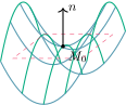
and $EG - F^2 = 1 + u^2 + v^2 > 0$ : regular everywhere. The two coordinate curves through a point are straight lines of $\R^3$ (fix $u$ or fix $v$ : the rulings of the doubly ruled saddle), yet $F \neq 0$ off the axes: rulings through a generic point are not orthogonal. Both rulings lie in the tangent plane, which they span — so the tangent plane cuts the surface along two whole lines, the extreme opposite of the sphere, whose tangent planes touch at one point only. The sign of the “second-order contact” between a surface and its tangent planes is a curvature story, taken up in the Year 3 volume.

Proposition 19.16 (Length of a curve drawn on a surface)

If $\gamma(t) = \sigma(u(t), v(t))$ , $t \in [a, b]$ , is $\mathcal{C}^1$ , then

L(\gamma) = \int_a^b \sqrt{E\,u'^2 + 2F\,u'v' + G\,v'^2}\;\dd t ,

with $E, F, G$ evaluated at $(u(t), v(t))$ .

Proof. $\gamma' = u'\sigma_u + v'\sigma_v$ by the chain rule, so $\norm{\gamma'}^2 = I(u', v') = Eu'^2 + 2Fu'v' + Gv'^2$ ; integrate $\norm{\gamma'}$ (Definition 18.6). ∎

Example 19.17 (Why airliners fly over the pole)

Two airports sit at latitude $\varphi_0$ and opposite longitudes: $A = \sigma(0, \varphi_0)$ and $B = \sigma(\pi, \varphi_0)$ on the sphere of radius $R$ . Along the parallel ( $\varphi \equiv \varphi_0$ ), the length is $\int_0^\pi R\cos\varphi_0\,\dd\theta = \pi R\cos\varphi_0$ . Along the route over the pole (up the meridian $\theta = 0$ , down the meridian $\theta = \pi$ ), it is $2R(\frac\pi2 - \varphi_0)$ . At latitude $\varphi_0 = \frac\pi3$ (sixty degrees): parallel route $\pi R/2 \approx 1.571\,R$ , polar route $\pi R/3 \approx 1.047\,R$ — a third shorter. In fact $\pi\cos\varphi_0 \geq \pi - 2\varphi_0$ on $\intcc0{\pi/2}$ (the function $\pi\cos\varphi - \pi + 2\varphi$ vanishes at both ends and its derivative $2 - \pi\sin\varphi$ changes sign once, so it is first increasing then decreasing, hence nonnegative): the polar route never loses. The first fundamental form turned a navigation question into two one-line integrals; Exercise 19.6 pushes the idea to a genuine minimality proof for meridians.

Lemma 19.18 (Lagrange identity)

For all $a, b \in \R^3$ : $\norm{a \wedge b}^2 = \norm a^2 \norm b^2 - \langle a, b\rangle^2$ . In particular

\norm{\sigma_u \wedge \sigma_v} = \sqrt{EG - F^2}.

Proof. Both sides are unchanged if we replace $b$ by its component $b_\perp = b - \frac{\langle a, b\rangle}{\norm a^2}a$ orthogonal to $a$ (for $a \neq 0$ ; the case $a = 0$ is trivial): the left side because $a \wedge a = 0$ , the right side by expanding $\norm {b_\perp}^2 = \norm b^2 - \frac{\langle a,b\rangle^2}{\norm a^2}$ and $\langle a, b_\perp\rangle = 0$ . So it suffices to prove the identity for orthogonal $a, b$ , where it reads $\norm{a \wedge b} = \norm a \norm b$ : true, since for orthogonal vectors the cross product has norm $\norm a\norm b\,\abs{\sin\frac\pi2}$ . The displayed formula is the case $a = \sigma_u$ , $b = \sigma_v$ . ∎

Remark 19.19

The Lagrange identity says $EG - F^2 = \det\left(\begin{smallmatrix} E & F\\ F & G\end{smallmatrix}\right)$ is the Gram determinant of $(\sigma_u, \sigma_v)$ : the squared area of the parallelogram they span. Regularity, positive definiteness of the first fundamental form, and positivity of the Gram determinant are three phrasings of one condition — which is why the area integrand below never vanishes on a regular chart.

Definition 19.20 (Area)

Let $\sigma \colon U \to \R^3$ be a regular injective $\mathcal{C}^1$ surface and $K \subseteq U$ a compact domain on which double integrals make sense (Chapter 20). The area of the piece $\sigma(K)$ is

\mathcal{A} = \iint_K \norm{\sigma_u \wedge \sigma_v}\,\dd u\,\dd v = \iint_K \sqrt{EG - F^2}\;\dd u\,\dd v .

Remark 19.21 (Why this formula)

The rectangle $[u, u + \dd u] \times [v, v + \dd v]$ is mapped, to first order, onto the parallelogram spanned by $\sigma_u\,\dd u$ and $\sigma_v\,\dd v$ , whose area is $\norm{\sigma_u \wedge \sigma_v}\,\dd u\,\dd v$ : the definition integrates the local area-distortion factor, exactly as arc length integrates the local speed. Consistency with change of parameters is Exercise 19.8; consistency with the change-of-variables formula for double integrals is discussed in Chapter 20.

Example 19.22 (Two different graphs, one area)

Over the unit disk, compare the bowl $z = \frac12(x^2 + y^2)$ and the saddle $z = xy$ . Their area integrands (Exercise 19.5) are

\sqrt{1 + x^2 + y^2} \qquad\text{and}\qquad \sqrt{1 + y^2 + x^2} :

identical. The two surfaces — one curving the same way in all directions, the other saddle-shaped — have exactly equal areas over every domain, $\frac{2\pi}3(2\sqrt2 - 1)$ over the unit disk. The area element only sees the length of the gradient, not the arrangement of the bending; telling the bowl from the saddle requires second-order data (the sign structure exhibited in Figure 19.1), which no amount of area measurement detects. First fundamental form: metric, blind to shape; the shape-seeing second form belongs to Year 3.

Example 19.23 (Area of the sphere)

For the spherical chart of Example 19.2:

\sigma_\theta = R(-\sin\theta\cos\varphi,\ \cos\theta\cos\varphi,\ 0), \qquad \sigma_\varphi = R(-\cos\theta\sin\varphi,\ -\sin\theta\sin\varphi,\ \cos\varphi),

so $E = R^2\cos^2\varphi$ , $F = 0$ , $G = R^2$ and $\sqrt{EG - F^2} = R^2\cos\varphi$ . Hence

\mathcal{A} = \int_{-\pi/2}^{\pi/2}\!\!\int_0^{2\pi} R^2\cos\varphi\;\dd\theta\,\dd\varphi = 2\pi R^2\,\bigl[\sin\varphi\bigr]_{-\pi/2}^{\pi/2} = \boxed{4\pi R^2} .

Example 19.24 (The cone, checked against the school formula)

For the cone $z = \sqrt{x^2 + y^2}$ over the annulus $a \leq \rho \leq b$ , the graph formula of Exercise 19.5 gives $1 + f_x^2 + f_y^2 = 2$ (compute $f_x = x/\rho$ , $f_y = y/\rho$ ), so

\mathcal A = \sqrt2\,\pi\,(b^2 - a^2) .

Consistency check with the slant-height formula $\pi\rho\ell$ of Example 19.26: the full cones of base radii $b$ and $a$ have lateral areas $\pi b\cdot b\sqrt2$ and $\pi a\cdot a\sqrt2$ , whose difference is exactly $\sqrt2\pi(b^2 - a^2)$ . Two charts, two formulas, one area — the invariance proved in Exercise 19.8, seen in the wild.

Remark 19.25 (Sanity checks for areas)

Three instant checks catch most errors in an area computation. Scaling: dilating a surface by $\lambda$ multiplies $E, F, G$ by $\lambda^2$ and the area by $\lambda^2$ — an answer whose dependence on $R$ is not quadratic (like $4\pi R^2$ ) is wrong. Positivity of the element: $\sqrt{EG - F^2}$ must be strictly positive on the chart’s interior; a vanishing value flags a chart degeneracy, to be excised as in the sphere’s poles. Symmetry: a computation over a symmetric piece must be consistent with summing its congruent parts — the hemisphere had better give $2\pi R^2$ .

Example 19.26 (Surface of revolution)

Rotate the curve $z \mapsto (r(z), 0, z)$ , $r > 0$ of class $\mathcal{C}^1$ , around the $z$ -axis:

\sigma(\theta, z) = (r(z)\cos\theta,\ r(z)\sin\theta,\ z).

Then $E = r(z)^2$ , $F = 0$ , $G = 1 + r'(z)^2$ , so

\mathcal{A} = \int_a^b\!\!\int_0^{2\pi} r(z)\sqrt{1 + r'(z)^2}\;\dd\theta\,\dd z = 2\pi\int_a^b r(z)\sqrt{1 + r'(z)^2}\,\dd z ,

the classical formula (circumference $2\pi r$ times the slant length element). For the cone $r(z) = kz$ , $z \in [0, h]$ : $\mathcal A = 2\pi k\sqrt{1 + k^2}\,\frac{h^2}{2} = \pi \rho \ell$ with $\rho = kh$ the base radius and $\ell = h\sqrt{1 + k^2}$ the slant height — the school formula, now derived rather than admitted.

Example 19.27 (The catenoid)

Rotate the catenary $r(z) = \cosh z$ , $z \in \intcc{-1}{1}$ , around its axis: the resulting catenoid has, by the revolution formula and $1 + \sinh^2 z = \cosh^2 z$ ,

\mathcal A = 2\pi\int_{-1}^1\cosh z\,\sqrt{1 + \sinh^2z}\, \dd z = 2\pi\int_{-1}^1\cosh^2z\,\dd z = \pi\bigl[z + \sinh z\cosh z\bigr]_{-1}^{1},

that is

\mathcal A = 2\pi + \pi\sinh 2 \approx 17.68 .

The slant factor $\sqrt{1 + r'^2}$ merged with the radius into a perfect square — the same identity that made the catenary’s arc length elementary in the curves chapter. This is no accident of algebra: among all surfaces of revolution spanning the two boundary circles, the catenoid minimizes area (it is the shape of a soap film between two rings), and this variational property is precisely what singles out $\cosh$ ; the Year 3 volume proves it with the calculus of variations.

The saddle z = x2 - y2 near the origin, with its coordinate curves (u-curves in blue, v-curves in green), the tangent plane at M_0 = (0,0,0) (dashed) and the unit normal n. The surface crosses its tangent plane — the two-dimensional analogue of an inflection. — **Figure 19.1.** The saddle $z = x^2 - y^2$ near the origin, with its coordinate curves ( $u$ -curves in blue, $v$ -curves in green), the tangent plane at $M_0 = (0,0,0)$ (dashed) and the unit normal $n$ . The surface crosses its tangent plane — the two-dimensional analogue of an inflection.

Remark 19.28 (Common pitfalls)

(i) Chart singularities are not surface singularities: the spherical chart degenerates at the poles ( $\cos\varphi = 0$ ), but the sphere is perfectly smooth there — another chart (exchange the roles of the axes) is regular at the poles. Before declaring a point singular, try a second parametrization. (ii) Regularity of $\sigma$ concerns the parametrization, not the image: $\sigma(u, v) = (u^3, v, 0)$ is non-regular along $u = 0$ although its image is a plane. (iii) The area formula requires $\sigma$ injective on $K$ : a chart covering a piece twice counts it twice ( $\theta$ running over $\intcc0{4\pi}$ doubles the sphere’s area). (iv) The unit normal is defined up to sign by the surface but is chosen by the chart (order of $u, v$ ); statements involving orientation must fix that choice. (v) Finally, $EG - F^2 > 0$ is not an extra hypothesis: it is exactly regularity, by the Lagrange identity — if it vanishes somewhere, the problem is the chart, and no area or tangent-plane formula applies there.

Remark 19.29 (Perspectives within this volume)

Forward links from here. The area element $\sqrt{EG - F^2}\,\dd u\,\dd v$ is a two-dimensional Jacobian in disguise, and Chapter 20 makes the analogy exact with the change-of-variables theorem — the surface integrals there are this chapter’s areas with an integrand on board. The first fundamental form is a field of positive quadratic forms, handled pointwise by the tools of Chapter 12, whose spectral theorem also powers this chapter’s weekend classification of quadrics. And the normal line drives extremum problems on constraint sets (Example 19.10), the geometric germ of the Lagrange multiplier method sketched with Theorem 15.11.

Four of the nine quadric surfaces classified in the weekend problem, sketched by their silhouettes and a level curve (red): the bounded ellipsoid, the doubly ruled one-sheet hyperboloid with its waist, the bowl of the elliptic paraboloid, and the saddle, whose two parabolic sections bend in opposite directions.

Remark 19.30 (Where this is used)

The area element $\norm{\sigma_u\wedge\sigma_v}\,\dd u\,\dd v$ is the surface-integral measure of Chapter 20, where it meets Green’s formula; the first fundamental form is the prototype of a field of quadratic forms, studied pointwise with the tools of Chapter 12; and this chapter’s weekend problem classifies all quadric surfaces with the spectral theorem. The Year 3 volume returns to surfaces with differential forms and the divergence theorem, and intrinsic curvature — what $E, F, G$ know about bending — is the gateway to differential geometry proper.

19.4 Exercises

Exercise 19.1 ★

Show that the tangent planes of the cone $z = \sqrt{x^2 + y^2}$ (minus its apex) all pass through the apex. (Parametrize by $\sigma(\theta, r) = (r\cos\theta, r\sin\theta, r)$ , $r > 0$ .)

Solution

Solution of Exercise 19.1.

With $\sigma(\theta, r) = (r\cos\theta,\ r\sin\theta,\ r)$ :

\sigma_\theta = (-r\sin\theta,\ r\cos\theta,\ 0), \qquad \sigma_r = (\cos\theta,\ \sin\theta,\ 1),

independent for $r > 0$ . The tangent plane at $M_0 = \sigma(\theta_0, r_0)$ passes through $M_0$ with directions $\sigma_\theta, \sigma_r$ . Now $M_0 - O = r_0(\cos\theta_0, \sin\theta_0, 1) = r_0\,\sigma_r(\theta_0, r_0)$ is itself a tangent direction: the apex $O$ lies on the tangent plane. (This is the general behaviour of cones: they are ruled by lines through the apex, and a tangent plane contains the ruling line through the point of tangency.)

Exercise 19.2 ★

Find the tangent plane of the ellipsoid $\frac{x^2}{a^2} + \frac{y^2}{b^2} + \frac{z^2}{c^2} = 1$ at a point $(x_0, y_0, z_0)$ of the surface.

Solution

Solution of Exercise 19.2.

Apply Proposition 19.7 to $f(x,y,z) = \frac{x^2}{a^2} + \frac{y^2}{b^2} + \frac{z^2}{c^2}$ : $\nabla f(x_0,y_0,z_0) = 2\bigl(\frac{x_0}{a^2}, \frac{y_0}{b^2}, \frac{z_0}{c^2}\bigr) \neq 0$ on the surface. The tangent plane is

\frac{x_0}{a^2}(x - x_0) + \frac{y_0}{b^2}(y - y_0) + \frac{z_0}{c^2}(z - z_0) = 0, \qquad\text{i.e.}\qquad \frac{x_0\,x}{a^2} + \frac{y_0\,y}{b^2} + \frac{z_0\,z}{c^2} = 1,

using that $(x_0, y_0, z_0)$ satisfies the ellipsoid equation — the “split the squares” rule generalizing the sphere’s $\langle M_0, M \rangle = R^2$ .

Exercise 19.3 ★

Compute $E, F, G$ for the helicoid $\sigma(u, v) = (v\cos u,\ v\sin u,\ au)$ , $a > 0$ , and the area of the piece $0 \leq u \leq 2\pi$ , $0 \leq v \leq 1$ , as an integral (evaluate it using $\int\sqrt{v^2 + a^2}\,\dd v = \frac12\bigl(v\sqrt{v^2+a^2} + a^2\ln(v + \sqrt{v^2 + a^2})\bigr) + C$ ).

Solution

Solution of Exercise 19.3.

$\sigma_u = (-v\sin u,\ v\cos u,\ a)$ and $\sigma_v = (\cos u,\ \sin u,\ 0)$ , so

E = v^2 + a^2, \qquad F = 0, \qquad G = 1, \qquad \sqrt{EG - F^2} = \sqrt{v^2 + a^2} > 0

(the helicoid is regular everywhere, including on its axis $v = 0$ ). Area of the piece:

\mathcal{A} = \int_0^{2\pi}\!\!\int_0^1 \sqrt{v^2 + a^2}\;\dd v\,\dd u = 2\pi\cdot\frac12\Bigl[v\sqrt{v^2 + a^2} + a^2\ln\bigl(v + \sqrt{v^2 + a^2}\bigr)\Bigr]_0^1 ,

i.e. $\mathcal{A} = \pi\Bigl(\sqrt{1 + a^2} + a^2\ln\frac{1 + \sqrt{1 + a^2}}{a}\Bigr)$ .

Exercise 19.4 ★★

(Torus) Parametrize the torus obtained by rotating the circle of center $(R, 0, 0)$ and radius $r < R$ in the $xz$ -plane around the $z$ -axis:

\sigma(\theta, \psi) = \bigl((R + r\cos\psi)\cos\theta,\ (R + r\cos\psi)\sin\theta,\ r\sin\psi\bigr).

Compute $E, F, G$ , check regularity, and show that the area is $4\pi^2 R r$ (Pappus: mean circumference $2\pi R$ times circle length $2\pi r$ ).

Solution

Solution of Exercise 19.4.

Derivatives:

\sigma_\theta = \bigl(-(R + r\cos\psi)\sin\theta,\ (R + r\cos\psi)\cos\theta,\ 0\bigr), \qquad \sigma_\psi = \bigl(-r\sin\psi\cos\theta,\ -r\sin\psi\sin\theta,\ r\cos\psi\bigr).

Then

E = (R + r\cos\psi)^2, \qquad F = r\sin\psi\cos\psi\,(R + r\cos\psi) \bigl(\sin\theta\cos\theta - \sin\theta\cos\theta\bigr) = 0, \qquad G = r^2 ,

so $\sqrt{EG - F^2} = r(R + r\cos\psi) \geq r(R - r) > 0$ : regular everywhere. Area:

\mathcal{A} = \int_0^{2\pi}\!\!\int_0^{2\pi} r(R + r\cos\psi) \,\dd\theta\,\dd\psi = 2\pi r \Bigl(2\pi R + r\int_0^{2\pi}\cos\psi\,\dd\psi\Bigr) = 4\pi^2 R r ,

the $\cos\psi$ term integrating to zero — Pappus’ theorem: area $=$ (length of the rotated circle) $\times$ (distance travelled by its center).

Exercise 19.5 ★★

Show that the area of the graph of $f \in \mathcal{C}^1(K)$ is $\iint_K \sqrt{1 + f_x^2 + f_y^2}\,\dd x\,\dd y$ , and compute it for the paraboloid piece $z = \frac12(x^2 + y^2)$ over the disk $x^2 + y^2 \leq 1$ (polar coordinates, Chapter 20).

Solution

Solution of Exercise 19.5.

For $\sigma(x, y) = (x, y, f(x,y))$ : $\sigma_x = (1, 0, f_x)$ , $\sigma_y = (0, 1, f_y)$ , so $E = 1 + f_x^2$ , $F = f_xf_y$ , $G = 1 + f_y^2$ and

EG - F^2 = (1 + f_x^2)(1 + f_y^2) - f_x^2f_y^2 = 1 + f_x^2 + f_y^2 ,

giving the stated area formula. For $f = \frac12(x^2 + y^2)$ on the unit disk: $1 + f_x^2 + f_y^2 = 1 + x^2 + y^2$ , and in polar coordinates ( $x = \rho\cos\alpha$ , $y = \rho\sin\alpha$ , Jacobian $\rho$ , Chapter 20):

\mathcal{A} = \int_0^{2\pi}\!\!\int_0^1 \sqrt{1 + \rho^2}\;\rho \,\dd\rho\,\dd\alpha = 2\pi\Bigl[\tfrac13(1 + \rho^2)^{3/2}\Bigr]_0^1 = \frac{2\pi}{3}\bigl(2\sqrt2 - 1\bigr).

Exercise 19.6 ★★

A drawn curve $\gamma(t) = \sigma(u(t), v(t))$ on the sphere of radius $R$ (spherical chart) has $u = \theta(t)$ , $v = \varphi(t)$ . Write its length as an integral in $\theta, \varphi$ and prove that among curves joining two points of the same meridian $\theta = \theta_0$ , the meridian arc is the shortest. (Bound the integrand below by $R\abs{\varphi'}$ .)

Solution

Solution of Exercise 19.6.

From Example 19.23’s computation, $E = R^2\cos^2\varphi$ , $F = 0$ , $G = R^2$ , so by Proposition 19.16

L = \int_a^b R\sqrt{\cos^2\varphi(t)\,\theta'(t)^2 + \varphi'(t)^2}\;\dd t .

Let the endpoints be $(\theta_0, \varphi_1)$ and $(\theta_0, \varphi_2)$ , $\varphi_1 < \varphi_2$ . For any joining curve,

L \geq \int_a^b R\,\abs{\varphi'(t)}\,\dd t \geq R\,\Bigl|\int_a^b \varphi'(t)\,\dd t\Bigr| = R\,(\varphi_2 - \varphi_1),

dropping the nonnegative $\cos^2\varphi\,\theta'^2$ term and using the triangle inequality for integrals. The meridian arc $\theta \equiv \theta_0$ , $\varphi$ increasing from $\varphi_1$ to $\varphi_2$ , has length exactly $R(\varphi_2 - \varphi_1)$ : it is shortest. (Meridians are great circles; this is the first, elementary case of the fact that geodesics of the sphere are great circles.)

Exercise 19.7 ★★★

(Normal lines of a sphere) Let $S$ be a regular level surface $\{f = c\}$ , connected, all of whose normal lines pass through a fixed point $\Omega$ . Show that $S$ is contained in a sphere centered at $\Omega$ . (Show that $\norm{M - \Omega}^2$ has zero derivative along every curve drawn on $S$ .)

Solution

Solution of Exercise 19.7.

Fix a curve $\gamma$ drawn on $S$ and let $g(t) = \norm{\gamma(t) - \Omega}^2$ . Then $g'(t) = 2\langle \gamma'(t),\ \gamma(t) - \Omega\rangle$ . The normal line at $M = \gamma(t)$ passes through $\Omega$ by hypothesis, so $\gamma(t) - \Omega$ is a normal vector, orthogonal to the tangent plane, in particular to the velocity $\gamma'(t)$ (Proposition 19.5): $g' = 0$ , and $g$ is constant along every drawn curve.

Now the set $S_c = \{M \in S : \norm{M - \Omega}^2 = c\}$ is closed in $S$ ; it is also open in $S$ : near any of its points, $S$ is a regular graph, so any nearby point of $S$ is joined to it by a drawn curve (a lifted segment), along which $g$ is constant. As $S$ is connected and $S_c$ nonempty for the right $c$ , $S = S_c \subseteq$ the sphere of center $\Omega$ and radius $\sqrt c$ (Chapter 4: connectedness argument).

Exercise 19.8 ★★★

(Area is geometric) Let $\Phi \colon U' \to U$ be a $\mathcal{C}^1$ diffeomorphism between open sets of $\R^2$ and $\tilde\sigma = \sigma \circ \Phi$ . Show that

\norm{\tilde\sigma_{u'} \wedge \tilde\sigma_{v'}} = \abs{\det J_\Phi}\, \norm{(\sigma_u \wedge \sigma_v)\circ\Phi} ,

and deduce, using the change-of-variables formula of Chapter 20, that the area of Definition 19.20 does not depend on the chosen regular parametrization.

Solution

Solution of Exercise 19.8.

Write $\Phi(u', v') = (u, v)$ . By the chain rule,

\tilde\sigma_{u'} = \frac{\partial u}{\partial u'}\sigma_u + \frac{\partial v}{\partial u'}\sigma_v, \qquad \tilde\sigma_{v'} = \frac{\partial u}{\partial v'}\sigma_u + \frac{\partial v}{\partial v'}\sigma_v ,

partials of $\sigma$ evaluated at $\Phi(u',v')$ . Expanding the cross product bilinearly and using $\sigma_u \wedge \sigma_u = \sigma_v \wedge \sigma_v = 0$ , $\sigma_v \wedge \sigma_u = -\sigma_u \wedge \sigma_v$ :

\tilde\sigma_{u'} \wedge \tilde\sigma_{v'} = \Bigl(\frac{\partial u}{\partial u'} \frac{\partial v}{\partial v'} - \frac{\partial v}{\partial u'} \frac{\partial u}{\partial v'}\Bigr)\, \sigma_u \wedge \sigma_v = \det J_\Phi \cdot (\sigma_u \wedge \sigma_v)\circ\Phi .

Taking norms gives the identity. Then, by the change-of-variables formula (Chapter 20) applied to the map $\Phi$ on $K' = \Phi^{-1}(K)$ :

\iint_{K'} \norm{\tilde\sigma_{u'} \wedge \tilde\sigma_{v'}} \,\dd u'\dd v' = \iint_{K'} \norm{\sigma_u \wedge \sigma_v}\circ\Phi\; \abs{\det J_\Phi}\,\dd u'\dd v' = \iint_K \norm{\sigma_u \wedge \sigma_v}\,\dd u\,\dd v :

the two parametrizations assign the same area to the same piece of surface.

Exercise 19.9 ★

(Archimedes’ hat-box theorem) On the sphere of radius $R$ , the zone between the latitudes with $z_1 \leq z \leq z_2$ ( $-R \leq z_1 < z_2 \leq R$ ) has area $2\pi R\,(z_2 - z_1)$ : prove it with the spherical chart, and conclude that a zone’s area depends only on its height — slicing an orange into equal-thickness slices gives equal amounts of peel.

Solution

Solution of Exercise 19.9.

In the spherical chart, $z = R\sin\varphi$ , and the zone corresponds to $\varphi_1 \leq \varphi \leq \varphi_2$ with $z_i = R\sin\varphi_i$ . With the area element $R^2\cos\varphi\,\dd\theta\,\dd\varphi$ (Example 19.23):

\mathcal A = \int_{\varphi_1}^{\varphi_2}\!\!\int_0^{2\pi} R^2\cos\varphi\,\dd\theta\,\dd\varphi = 2\pi R^2(\sin\varphi_2 - \sin\varphi_1) = 2\pi R\,(z_2 - z_1) .

The result depends only on the height $z_2 - z_1$ : slices of equal thickness carry equal areas, whether cut at the equator or at the pole — Archimedes’ hat-box theorem, and the reason the lateral area of the circumscribed cylinder ( $2\pi R \cdot 2R = 4\pi R^2$ ) equals the area of the sphere.

Exercise 19.10 ★★

Show that every normal line of a surface of revolution $\sigma(\theta, z) = (r(z)\cos\theta,\ r(z)\sin\theta,\ z)$ ( $r > 0$ of class $\mathcal C^1$ ) meets the axis of revolution, and locate the intersection point.

Solution

Solution of Exercise 19.10.

$\sigma_\theta = (-r\sin\theta,\ r\cos\theta,\ 0)$ and $\sigma_z = (r'\cos\theta,\ r'\sin\theta,\ 1)$ , so

\sigma_\theta \wedge \sigma_z = (r\cos\theta,\ r\sin\theta,\ -r\,r') ,

a normal vector at $M = (r\cos\theta, r\sin\theta, z)$ . The normal line is

t \mapsto \bigl(r(1 + t)\cos\theta,\ r(1 + t)\sin\theta,\ z - t\,r\,r'\bigr),

which at $t = -1$ reaches $(0,\ 0,\ z + r(z)\,r'(z))$ : every normal line meets the axis, at the height $z + rr'$ . (This is the three-dimensional reason rotational symmetry survives in the normal field.)

Exercise 19.11 ★★

(Unrolling the cylinder) The chart $\sigma(u, v) = (\cos u,\ \sin u,\ v)$ of the unit cylinder has $E = G = 1$ , $F = 0$ : verify this, and explain why every drawn curve $t \mapsto \sigma(u(t), v(t))$ has the same length as the plane curve $t \mapsto (u(t), v(t))$ . Deduce that the helix from $(1, 0, 0)$ to $(1, 0, 2\pi c)$ making one turn has length $2\pi\sqrt{1 + c^2}$ , and that no drawn curve with the same endpoints and one full turn is shorter.

Solution

Solution of Exercise 19.11.

$\sigma_u = (-\sin u, \cos u, 0)$ , $\sigma_v = (0, 0, 1)$ : $E = 1$ , $F = 0$ , $G = 1$ . By Proposition 19.16 the length of a drawn curve is $\int\sqrt{u'^2 + v'^2}\,\dd t$ — the length of its parameter shadow $(u(t), v(t))$ in the plane: the chart is a local isometry (the unrolling of the cylinder). The helix $t \mapsto (\cos t, \sin t, ct)$ , $t \in \intcc0{2\pi}$ , has shadow the segment from $(0,0)$ to $(2\pi, 2\pi c)$ , of length $2\pi\sqrt{1 + c^2}$ . Any drawn curve from $(1,0,0)$ to $(1, 0, 2\pi c)$ making one full turn has a continuous shadow joining $(0, 0)$ to $(2\pi, 2\pi c)$ , of plane length $\geq$ the straight segment; since lengths agree, the helix is shortest.

Exercise 19.12 ★★★

Let $S = \{f = c\}$ be a compact regular level surface and $M_0 \in S$ a point at maximal distance from the origin. Show that $\nabla f(M_0)$ is collinear with $\vect{OM_0}$ — the normal at the farthest point is radial. Apply to the ellipsoid $\frac{x^2}{a^2} + \frac{y^2}{b^2} + \frac{z^2}{c^2} = 1$ ( $a > b > c > 0$ ): find all points where the normal is radial, and identify the farthest ones.

Solution

Solution of Exercise 19.12.

The function $g(M) = \norm{M}^2$ is continuous on the compact $S$ , so it attains its maximum at some $M_0$ . For every curve $\gamma$ drawn on $S$ with $\gamma(0) = M_0$ , the function $t \mapsto \norm{\gamma(t)}^2$ has a maximum at $t = 0$ , so its derivative $2\langle\gamma'(0), M_0\rangle$ vanishes: $M_0$ is orthogonal to every tangent vector, i.e. normal to $S$ at $M_0$ . As $\nabla f(M_0) \neq 0$ also directs the normal line (Proposition 19.7), $\nabla f(M_0)$ and $\vect{OM_0}$ are collinear. For the ellipsoid, radiality means

\Bigl(\frac{x_0}{a^2}, \frac{y_0}{b^2}, \frac{z_0}{c^2}\Bigr) = \mu\,(x_0, y_0, z_0) :

each coordinate satisfies $x_0(\frac1{a^2} - \mu) = 0$ , etc.; since $a^{-2}, b^{-2}, c^{-2}$ are distinct, at most one coordinate is nonzero, and the solutions on the surface are the six axis endpoints $(\pm a, 0, 0)$ , $(0, \pm b, 0)$ , $(0, 0, \pm c)$ . The farthest points are $(\pm a, 0, 0)$ , at distance $a = \max(a,b,c)$ .

19.5 Problem: the classification of quadrics of $\R^3$

Problem 19.1

Weekend problem — every quadric surface, sorted by the spectral theorem

A quadric is the zero set in $\R^3$ of a degree-two polynomial

q(X) = X^{\mathsf T}\!AX + 2\,\langle b, X\rangle + c, \qquad A \in \mathcal S_3(\R),\ A \neq 0,\ b \in \R^3,\ c \in \R .

The surfaces of this chapter’s figures — spheres, ellipsoids, saddles, cones, cylinders — are all quadrics. This problem classifies them all: the spectral theorem (Theorem 12.13) straightens the quadratic part, affine translations (Chapter 17) absorb the linear part, and what remains is a short, complete list of normal forms.

Part I — The reduction machine.

Let $X = PY + t$ with $P \in O(3)$ and $t \in \R^3$ (a rigid change of coordinates). Show that $q(PY + t) = Y^{\mathsf T}\!A'Y + 2\langle b', Y\rangle + c'$ with

$A' = P^{\mathsf T}\!AP, \qquad b' = P^{\mathsf T}(At + b), \qquad c' = q(t) .$

Deduce that the spectrum of $A$ (hence its rank and signature) is a rigid invariant of the equation, and explain why the equation of a given quadric is only determined up to a nonzero scalar factor.
Using the spectral theorem, show that after a rotation the equation becomes $\sum_i \lambda_i y_i^2 + 2\sum_i\beta_iy_i + c = 0$ with $\lambda_1, \lambda_2, \lambda_3$ the eigenvalues of $A$ .
For every $i$ with $\lambda_i \neq 0$ , absorb $\beta_iy_i$ by a translation ( $y_i \mapsto y_i - \beta_i/\lambda_i$ ). Write the reduced equation when $\operatorname{rank} A = r$ : $\sum_{i\leq r}\lambda_i z_i^2 + 2\sum_{i > r}\beta_iz_i + c'' = 0$ .
A center of the quadric of equation $q = 0$ is a point $\Omega$ with $q(2\Omega - X) = q(X)$ for all $X$ : the point reflection in $\Omega$ preserves the equation, hence the surface. Show that $q(2\Omega - X) - q(X) = -4\langle A\Omega + b, X\rangle + 4\langle A\Omega + b, \Omega\rangle$ , and deduce: the centers are exactly the solutions of $A\Omega = -b$ ; they exist iff $b \in \operatorname{im}A$ , and the center is unique iff $A$ is invertible.

Part II — Central quadrics ( $\operatorname{rank}A = 3$ ). Here the reduced equation is $\lambda_1z_1^2 + \lambda_2z_2^2 + \lambda_3z_3^2 = \delta$ .

Multiplying by $-1$ if needed, assume at least two $\lambda_i > 0$ . Enumerate the possibilities: signature $(3, 0)$ with $\delta > 0$ , $= 0$ , $< 0$ , and signature $(2, 1)$ with $\delta > 0$ , $= 0$ , $< 0$ ; name the six resulting sets (ellipsoid, point, empty set, one-sheet hyperboloid, cone, two-sheet hyperboloid) and put each in its Euclidean normal form ( $\frac{x^2}{a^2} + \frac{y^2}{b^2} + \frac{z^2}{c^2} = 1$ , etc.).
Classify $x^2 + y^2 + z^2 + 4xy + 4yz + 4zx = 1$ : show $A = 2J - I$ with $J$ the all-ones matrix, compute the spectrum $\{5, -1, -1\}$ , and identify a two-sheet hyperboloid of revolution about the axis $\R(1,1,1)$ .
(Rulings) For the one-sheet hyperboloid $\frac{x^2}{a^2} + \frac{y^2}{b^2} - \frac{z^2}{c^2} = 1$ , factor

$\Bigl(\frac xa - \frac zc\Bigr) \Bigl(\frac xa + \frac zc\Bigr) = \Bigl(1 - \frac yb\Bigr)\Bigl(1 + \frac yb\Bigr)$

and produce two one-parameter families of straight lines lying on the surface.
Show that through every point of the one-sheet hyperboloid passes exactly one line of each family: the surface is doubly ruled.
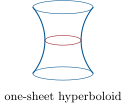
The asymptotic cone of the one-sheet hyperboloid is $C : \frac{x^2}{a^2} + \frac{y^2}{b^2} - \frac{z^2}{c^2} = 0$ . With $\rho^2 = \frac{x^2}{a^2} + \frac{y^2}{b^2}$ , show that any point of the hyperboloid is at distance at most $c\bigl(\rho - \sqrt{\rho^2 - 1}\bigr) = \frac{c}{\rho + \sqrt{\rho^2 - 1}}$ from $C$ , so the surface hugs its cone at infinity. What are the sections of the hyperboloid by the planes $x = \pm a$ ?

Part III — Rank $2$ and rank $1$ : paraboloids, cylinders, planes.

Suppose $\operatorname{rank}A = 2$ , say $\lambda_1, \lambda_2 \neq 0 = \lambda_3$ . Starting from question 3, split into two cases according to $\beta_3 \neq 0$ (no center, by question 4) or $\beta_3 = 0$ (a line of centers), and reduce to

$\lambda_1z_1^2 + \lambda_2z_2^2 + 2\beta_3z_3 = 0 \qquad\text{or}\qquad \lambda_1z_1^2 + \lambda_2z_2^2 + c'' = 0 :$

elliptic/hyperbolic paraboloids in the first case, cylinders over central conics (or pairs of intersecting planes, a line, the empty set) in the second.
Show that the saddle $z = xy$ is a hyperbolic paraboloid: rotate by $\pi/4$ in the $xy$ -plane to reach $z = \tfrac12(u^2 - v^2)$ , the surface of Figure 19.1 up to scale.
Show that the saddle $z = xy$ carries the two line families $\{x = x_0,\ z = x_0y\}$ and $\{y = y_0,\ z = xy_0\}$ , with exactly one line of each through every point: the second doubly ruled quadric.
Classify $x^2 + y^2 - 2x + 4y + 3 = 0$ in $\R^3$ (complete the squares; identify a right circular cylinder, and give its axis and radius).
Now let $\operatorname{rank}A = 1$ , say $\lambda_1 \neq 0 = \lambda_2 = \lambda_3$ . Rotating within the kernel plane and translating, reduce to

$\lambda_1z_1^2 + 2\beta z_2 = 0 \quad (\beta \neq 0) \qquad\text{or}\qquad \lambda_1z_1^2 + c'' = 0 :$

a parabolic cylinder, or a pair of parallel planes, a double plane, or the empty set. Classify $(x + y)^2 = z$ completely (normal form, axis of translation invariance).

Part IV — The classification theorem.

Assemble Parts I–III into a theorem: every quadric of $\R^3$ is mapped by a rigid motion onto exactly one normal form. List the seventeen affine types (count the empty variants and degenerate sets), and single out the nine quadric surfaces: ellipsoid, one- and two-sheet hyperboloids, cone, elliptic and hyperbolic paraboloids, elliptic, hyperbolic and parabolic cylinders.
Write the classification algorithm: given $(A, b, c)$ , which quantities do you compute, in which order, and which branch decides which type? Justify that each step is effective (eigenvalues of a symmetric $3\times3$ matrix, rank, solvability of $A\Omega = -b$ ).
Run the algorithm on $x^2 + y^2 + z^2 - 2xy - 2yz - 2zx = 1$ : show $A = 2I - J$ has spectrum $\{2, 2, -1\}$ and conclude: a one-sheet hyperboloid of revolution about $\R(1,1,1)$ .
Run it on $x^2 + y^2 - z^2 - 2x + 4y + 2z + 4 = 0$ : find the center and identify the quadric.
Run it on $x^2 + 4xy + y^2 = 2z$ : diagonalize the $xy$ -block ( $u = \frac{x+y}{\sqrt2}$ , $v = \frac{x-y}{\sqrt2}$ ) and identify the quadric.
Euclidean versus affine. Show that two central quadrics in normal form are rigidly equivalent iff they have the same coefficient lists (up to permutation and a common positive scalar on the equation), while affinely, only the signature data survives: every ellipsoid is an affine image of the round sphere. Which theorem guarantees that the signature cannot change along the way (Theorem 12.6)?

Part V — Dividends.

Show that every section of a quadric by an affine plane is a conic (possibly degenerate) of that plane. Identify the sections of the saddle $z = xy$ by the planes $z = c$ ( $c \neq 0$ and $c = 0$ ).
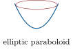
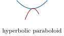
Which quadric surfaces contain straight lines? Show that the ellipsoid, the two-sheet hyperboloid and the elliptic paraboloid contain none (restrict $q$ to a line and use the Cauchy–Schwarz inequality for the two-sheet case); that cone and cylinders are ruled by one family; and conclude that the doubly ruled quadric surfaces are exactly the one-sheet hyperboloid and the hyperbolic paraboloid.
When only the affine type is wanted, Gauss’s reduction (Theorem 12.5) is cheaper than diagonalizing. Redo question 17 with Gauss’s algorithm and check the signature $(2, 1)$ ; what Euclidean information does Gauss lose?
All eigenvalues of a symmetric matrix are real; show that consequently the signs of the eigenvalues of $A$ can be read from the characteristic polynomial by Descartes’ rule of signs, and verify it on question 6: $\chi_A(\lambda) = \lambda^3 - 3\lambda^2 - 9\lambda - 5$ has exactly one sign change, hence signature $(1, 2)$ .
Synthesis. Summarize the algorithm in a few lines; state the exact role played by (i) the spectral theorem, (ii) the center equation $A\Omega = -b$ , (iii) Sylvester’s inertia theorem, (iv) Gauss’s reduction. What does the same machine yield in $\R^2$ , and what changes in $\R^n$ ?

Solution

Solution of Problem 19.1.

1. Expanding, and using the symmetry of $A$ ( $t^{\mathsf T}\!APY = (At)^{\mathsf T}PY$ ):

q(PY + t) = Y^{\mathsf T}P^{\mathsf T}\!APY + 2\,(At + b)^{\mathsf T}PY + \bigl(t^{\mathsf T}\!At + 2b^{\mathsf T}t + c\bigr),

which is the displayed triple. $A' = P^{\mathsf T}\!AP = P^{-1}AP$ is similar to $A$ : same characteristic polynomial, spectrum, rank, signature. Finally $\{q = 0\} = \{sq = 0\}$ for $s \neq 0$ , so only the equation up to a scalar is attached to the set; scaling by $s$ multiplies all eigenvalues by $s$ .

2. The spectral theorem provides $P \in O(3)$ with $P^{\mathsf T}\!AP = \operatorname{diag}(\lambda_1, \lambda_2, \lambda_3)$ ; question 1 with $t = 0$ turns the equation into $\sum\lambda_iy_i^2 + 2\sum\beta_iy_i + c = 0$ , where $\beta = P^{\mathsf T}b$ .

3. For $\lambda_i \neq 0$ : $\lambda_iy_i^2 + 2\beta_iy_i = \lambda_i\bigl(y_i + \frac{\beta_i}{\lambda_i}\bigr)^2 - \frac{\beta_i^2}{\lambda_i}$ ; the translation $z_i = y_i + \beta_i/\lambda_i$ (and $z_i = y_i$ for $i > r$ ) gives

\sum_{i \leq r}\lambda_iz_i^2 + 2\sum_{i > r}\beta_iz_i + c'' = 0, \qquad c'' = c - \sum_{i\leq r}\frac{\beta_i^2}{\lambda_i}.

4. $q(2\Omega - X) = (2\Omega - X)^{\mathsf T} A(2\Omega - X) + 2b^{\mathsf T}(2\Omega - X) + c$ ; expanding and subtracting $q(X)$ , the quadratic terms cancel and

q(2\Omega - X) - q(X) = -4\,\langle A\Omega + b,\ X\rangle + 4\,\langle A\Omega + b,\ \Omega\rangle .

If $A\Omega + b = 0$ this vanishes identically: the point reflection preserves $q$ , hence the quadric. Conversely, “ $q(2\Omega - X) = q(X)$ for all $X$ ” says that the affine function above vanishes on all of $\R^3$ , which forces its linear part $A\Omega + b$ to be zero. So centers $=$ solutions of $A\Omega = -b$ : a nonempty set iff $b \in \operatorname{im}A$ (an affine subspace directed by $\ker A$ ), and a single point iff $A$ is invertible.

5. Signature $(3,0)$ (all $\lambda_i > 0$ ): $\delta > 0$ gives $\frac{x^2}{a^2} + \frac{y^2}{b^2} + \frac{z^2}{c^2} = 1$ with $a = \sqrt{\delta/\lambda_1}$ , etc. — an ellipsoid; $\delta = 0$ : the single point $O$ ; $\delta < 0$ : empty. Signature $(2,1)$ ( $\lambda_1, \lambda_2 > 0 > \lambda_3$ ): $\delta > 0$ : $\frac{x^2}{a^2} + \frac{y^2}{b^2} - \frac{z^2}{c^2} = 1$ , the one-sheet hyperboloid; $\delta = 0$ : the cone $\frac{x^2}{a^2} + \frac{y^2}{b^2} = \frac{z^2}{c^2}$ ; $\delta < 0$ : $\frac{z^2}{c^2} - \frac{x^2}{a^2} - \frac{y^2}{b^2} = 1$ , the two-sheet hyperboloid ( $\abs z \geq c$ : two components).

6. The quadratic part has matrix $A$ with diagonal $1$ and off-diagonal $2$ : $A = 2J - I$ . Since $J$ has spectrum $\{3, 0, 0\}$ (eigenvector $(1,1,1)$ for $3$ ), $A$ has spectrum $\{5, -1, -1\}$ , the eigenvalue $5$ carried by $\R(1,1,1)$ . In the rotated coordinates: $5u^2 - v^2 - w^2 = 1$ , i.e. $\frac{u^2}{1/5} - v^2 - w^2 = 1$ : a two-sheet hyperboloid, of revolution (equal eigenvalues $-1$ ) about the axis $\R(1,1,1)$ .

7. The surface is $\bigl(\frac xa - \frac zc\bigr)\bigl(\frac xa + \frac zc\bigr) = \bigl(1 - \frac yb\bigr)\bigl(1 + \frac yb\bigr)$ . For $(\lambda : \mu) \neq (0:0)$ define the line

D_{\lambda:\mu} :\quad \lambda\Bigl(\frac xa - \frac zc\Bigr) = \mu\Bigl(1 - \frac yb\Bigr), \qquad \mu\Bigl(\frac xa + \frac zc\Bigr) = \lambda\Bigl(1 + \frac yb\Bigr)

(two independent affine equations: a line). Multiplying the two equations shows every point of $D_{\lambda:\mu}$ lies on the surface when $\lambda\mu \neq 0$ ; the cases $\lambda = 0$ or $\mu = 0$ are checked directly (e.g. $\lambda = 0$ : $y = b$ , $\frac xa = -\frac zc$ , which satisfies the equation). The second family $D'_{\lambda:\mu}$ swaps the two right-hand factors.

8. Fix $M$ on the surface. The conditions for $M \in D_{\lambda:\mu}$ form a $2\times2$ homogeneous linear system in $(\lambda, \mu)$ whose determinant is

\Bigl(\frac{x^2}{a^2} - \frac{z^2}{c^2}\Bigr) - \Bigl(1 - \frac{y^2}{b^2}\Bigr) = 0

precisely because $M$ lies on the quadric: a nontrivial solution $(\lambda : \mu)$ exists. The coefficient matrix is never zero (that would force $1 - \frac yb = 1 + \frac yb = 0$ ), so its rank is $1$ and the solution is unique up to scale: exactly one line of the family passes through $M$ . The same holds for the second family, and the two lines are distinct (at $(a, 0, 0)$ they are $\{x = a,\ \frac zc = \frac yb\}$ and $\{x = a,\ \frac zc = -\frac yb\}$ ): the one-sheet hyperboloid is doubly ruled.

9. Let $M = (x, y, z)$ on the hyperboloid, $\rho^2 = \frac{x^2}{a^2} + \frac{y^2}{b^2} = 1 + \frac{z^2}{c^2} \geq 1$ . The point $N = (x,\ y,\ \varepsilon c\rho)$ with $\varepsilon$ the sign of $z$ satisfies $\frac{x^2}{a^2} + \frac{y^2}{b^2} - \frac{(c\rho)^2}{c^2} = 0$ : $N \in C$ , and

d(M, C) \leq \abs{z - \varepsilon c\rho} = c\bigl(\rho - \sqrt{\rho^2 - 1}\bigr) = \frac{c}{\rho + \sqrt{\rho^2 - 1}} .

If $\norm M \to \infty$ then $\rho \to \infty$ (all three coordinates are bounded by multiples of $\rho$ ), so $d(M, C) \to 0$ . The section $x = a$ : $\frac{y^2}{b^2} - \frac{z^2}{c^2} = 0$ , the pair of crossing lines of question 8 — and likewise at $x = -a$ .

10. With $\lambda_3 = 0$ , question 3 leaves $\lambda_1z_1^2 + \lambda_2z_2^2 + 2\beta_3z_3 + c'' = 0$ . In the eigenbasis, $\operatorname{im}A = \operatorname{Vect}(e_1, e_2)$ , so by question 4 centers exist iff $\beta_3 = 0$ . If $\beta_3 \neq 0$ : the translation $z_3 \mapsto z_3 - c''/(2\beta_3)$ removes the constant, leaving $\lambda_1z_1^2 + \lambda_2z_2^2 + 2\beta_3z_3 = 0$ , i.e. $z_3 = px^2 + qy^2$ after renaming: an elliptic paraboloid if $\lambda_1\lambda_2 > 0$ , a hyperbolic paraboloid if $\lambda_1\lambda_2 < 0$ — and indeed no center. If $\beta_3 = 0$ : the equation $\lambda_1z_1^2 + \lambda_2z_2^2 + c'' = 0$ does not involve $z_3$ : the quadric is a cylinder over the corresponding plane conic — elliptic cylinder, line, or empty set when $\lambda_1\lambda_2 > 0$ ; hyperbolic cylinder or pair of intersecting planes when $\lambda_1\lambda_2 < 0$ — with a whole line of centers $\{(z_1^*, z_2^*)\} \times \R$ .

11. $xy - z = 0$ . Substituting $x = \frac{u + v}{\sqrt2}$ , $y = \frac{u - v}{\sqrt2}$ (rotation by $\pi/4$ ): $xy = \frac{u^2 - v^2}2$ , so the equation becomes $z = \frac12(u^2 - v^2)$ : a hyperbolic paraboloid — the saddle of the figure, up to the factor $\frac12$ .

12. The line $\{x = x_0,\ z = x_0y\}$ (parametrized by $y$ ) clearly lies on $z = xy$ , as does $\{y = y_0,\ z = xy_0\}$ ; through $(x_0, y_0, x_0y_0)$ pass the two of them. Uniqueness: if $t \mapsto (x_0 + tv_1, y_0 + tv_2, z_0 + tv_3)$ stays on the surface, the coefficient of $t^2$ in $(x_0 + tv_1)(y_0 + tv_2) - z_0 - tv_3$ gives $v_1v_2 = 0$ , so $v_1 = 0$ or $v_2 = 0$ , landing in one of the two families: one line of each through each point — the second doubly ruled quadric.

13. Completing squares: $(x - 1)^2 + (y + 2)^2 = 2$ , with no condition on $z$ : a right circular cylinder of radius $\sqrt2$ and axis the vertical line $\{(1, -2, z) : z \in \R\}$ — a line of centers, as question 10 predicts.

14. With $\lambda_2 = \lambda_3 = 0$ the reduced equation is $\lambda_1z_1^2 + 2\beta_2z_2 + 2\beta_3z_3 + c'' = 0$ . A rotation of the kernel plane $(z_2, z_3)$ aligns the linear form: $2\beta_2z_2 + 2\beta_3z_3 = 2\beta w$ with $\beta = \sqrt{\beta_2^2 + \beta_3^2}$ . If $\beta \neq 0$ , translate $w$ to absorb $c''$ : $\lambda_1z_1^2 + 2\beta w = 0$ , a parabolic cylinder; if $\beta = 0$ : $\lambda_1z_1^2 = -c''$ gives two parallel planes ( $c'' \lambda_1 < 0$ ), a double plane ( $c'' = 0$ ), or the empty set. For $(x + y)^2 = z$ : with $u = \frac{x + y}{\sqrt2}$ the equation reads $z = 2u^2$ : a parabolic cylinder, invariant under translations along $(1, -1, 0)$ .

15. Every quadric is carried by a rotation plus translations onto one of: (rank 3) ellipsoid, point, empty set, one-sheet hyperboloid, cone, two-sheet hyperboloid; (rank 2) elliptic paraboloid, hyperbolic paraboloid, elliptic cylinder, line, empty set, hyperbolic cylinder, pair of intersecting planes; (rank 1) parabolic cylinder, pair of parallel planes, double plane, empty set. Identifying the three empty variants as distinct affine types of equations, the count is seventeen; among them nine are honest surfaces: ellipsoid, the two hyperboloids, the cone, the two paraboloids, and the three cylinders.

16. Algorithm. (i) Read off $(A, b, c)$ ; compute the characteristic polynomial of $A$ , its eigenvalues (real, by the spectral theorem) and $r = \operatorname{rank}A$ . (ii) Solve $A\Omega = -b$ (Gaussian elimination): solvable or not — centers or not. (iii) If solvable, translate to a center: the equation becomes $\sum\lambda_iz_i^2 + c'' = 0$ with $c'' = c + \langle b, \Omega\rangle$ ; sort by $r$ , the signature, and the sign of $c''$ using questions 5, 10, 14. (iv) If not solvable ( $r \leq 2$ ), rotate and reduce as in questions 10 and 14: paraboloid ( $r = 2$ ) or parabolic cylinder ( $r = 1$ ), elliptic/hyperbolic according to the sign of $\lambda_1\lambda_2$ . Each step is a finite computation: roots of a cubic with real roots, ranks, linear systems.

17. $A$ has diagonal $1$ , off-diagonal $-1$ : $A = 2I - J$ , spectrum $\{2 - 3,\ 2,\ 2\} = \{-1, 2, 2\}$ with $-1$ on $\R(1,1,1)$ . Signature $(2,1)$ , $b = 0$ , right side $\delta = 1 > 0$ : $2u^2 + 2v^2 - w^2 = 1$ , a one-sheet hyperboloid of revolution about the axis $\R(1,1,1)$ .

18. Complete squares: $(x-1)^2 + (y+2)^2 - (z-1)^2 + (-1 - 4 + 1 + 4) = 0$ , i.e.

(x-1)^2 + (y+2)^2 = (z-1)^2 :

the constant vanished — a right circular cone with vertex (and unique center) $(1, -2, 1)$ and axis parallel to $Oz$ .

19. The quadratic part $x^2 + 4xy + y^2$ has matrix $\left(\begin{smallmatrix}1 & 2\\ 2 & 1\end{smallmatrix}\right)$ (in the $xy$ -plane), eigenvalues $3$ (on $(1,1)$ ) and $-1$ (on $(1,-1)$ ): with $u = \frac{x+y}{\sqrt2}$ , $v = \frac{x-y}{\sqrt2}$ it equals $3u^2 - v^2$ , and the quadric is

z = \tfrac32u^2 - \tfrac12v^2 :

a hyperbolic paraboloid ( $A$ has rank $2$ and $b$ has a component along $\ker A = \R e_z$ : no center).

20. A rigid motion transforms the equation’s data by $A \mapsto P^{\mathsf T}\!AP$ (same eigenvalues) and the normal forms have no residual freedom except permuting coordinates and multiplying the whole equation by a scalar ( $> 0$ to preserve the writing): two central normal forms coincide up to isometry iff the coefficient lists agree up to permutation and common positive factor — for the ellipsoid, iff the semiaxes $(a, b, c)$ agree. Affinely, one may also scale each coordinate separately ( $z_i \mapsto z_i\sqrt{\abs {\lambda_i}}$ ), which erases the eigenvalues and leaves only their signs: every ellipsoid becomes $u^2 + v^2 + w^2 = 1$ , the sphere. Sylvester’s inertia theorem (Theorem 12.6) guarantees the signature survives any invertible linear change: the affine types of question 15 are genuinely distinct.

21. Parametrize the plane affinely: $M = P + su + tv$ . Then $q(P + su + tv)$ is a polynomial of degree $\leq 2$ in $(s, t)$ (expand the quadratic form bilinearly), so the section $\{q = 0\}$ is a conic of the plane, possibly degenerate. For $z = xy$ and the plane $z = c$ : $xy = c$ , a hyperbola for $c \neq 0$ , and for $c = 0$ the two coordinate lines — the pair of rulings through the origin.

22. Ellipsoid: bounded, contains no line. Two-sheet hyperboloid $\frac{z^2}{c^2} - \frac{x^2}{a^2} - \frac{y^2}{b^2} = 1$ : restrict to $p + tv$ ; the $t^2$ coefficient $\frac{v_3^2}{c^2} - \frac{v_1^2}{a^2} - \frac{v_2^2}{b^2}$ must vanish, so $v_3 \neq 0$ (else $v = 0$ ); the $t$ coefficient gives $\frac{p_3v_3}{c^2} = \frac{p_1v_1}{a^2} + \frac{p_2v_2}{b^2}$ , and Cauchy–Schwarz yields

\frac{p_3^2}{c^2} = \frac{c^2}{v_3^2}\Bigl(\frac{p_1v_1}{a^2} + \frac{p_2v_2}{b^2}\Bigr)^2 \leq \frac{c^2}{v_3^2}\Bigl(\frac{p_1^2}{a^2} + \frac{p_2^2}{b^2}\Bigr)\frac{v_3^2}{c^2} = \frac{p_1^2}{a^2} + \frac{p_2^2}{b^2},

so the constant term is $\leq 0 \neq 1$ : no line. Elliptic paraboloid $z = \frac{x^2}{a^2} + \frac{y^2}{b^2}$ : the $t^2$ coefficient forces $v_1 = v_2 = 0$ , then the equation is linear nonconstant in $t$ : no line. Cone $x^2 + y^2 = z^2$ : a line on it satisfies $q(p) = q(v) = B(p, v) = 0$ for the Lorentz form; equality in the plane Cauchy–Schwarz $\abs{p_1v_1 + p_2v_2} = \abs{p_3v_3} = \sqrt{(p_1^2 + p_2^2)(v_1^2 + v_2^2)}$ forces $(p_1, p_2) \parallel (v_1, v_2)$ and then $p = kv$ : all lines pass through the vertex — one family. Cylinders: for the elliptic and parabolic cylinders the $t^2$ coefficient forces $v_1 = v_2 = 0$ (rulings only); for the hyperbolic cylinder $\frac{x^2}{a^2} - \frac{y^2}{b^2} = 1$ , $\frac{v_1}a = \pm \frac{v_2}b$ with $v_2 \neq 0$ leads via the $t$ coefficient to $\frac{p_1^2}{a^2} = \frac{p_2^2}{b^2}$ , contradicting the constant term $1$ : again only the vertical rulings. So the doubly ruled quadric surfaces are exactly the one-sheet hyperboloid and the hyperbolic paraboloid.

23. Gauss: $x^2 - 2xy - 2zx = (x - y - z)^2 - y^2 - z^2 - 2yz$ , so

q = (x - y - z)^2 - 4yz = (x - y - z)^2 + (y - z)^2 - (y + z)^2 :

three independent squares with signs $(+, +, -)$ — signature $(2, 1)$ , matching question 17, with no eigenvalue computation. Gauss loses the metric data: the new coordinates are not orthonormal, so the eigenvalues (the shape of the hyperboloid, its axes and their lengths) are gone; only the affine type remains.

24. Let $p$ , $n$ , $z$ be the numbers of positive, negative and zero eigenvalues, $p + n + z = 3$ . Descartes’ rule bounds $p$ by the number $V$ of sign changes of $\chi_A$ , and $n$ by the number $V'$ of sign changes of $\chi_A(-\lambda)$ ; moreover each pair of consecutive nonzero coefficients produces a change in exactly one of the two polynomials, so $V + V' \leq 3 - z$ (zero roots are visible as vanishing trailing coefficients). Then $p + n = 3 - z \geq V + V' \geq p + n$ : equality, so $p = V$ exactly — the signs of the eigenvalues can be read off. For $\chi_A(\lambda) = \lambda^3 - 3\lambda^2 - 9\lambda - 5$ : signs $+,-,-,-$ give $V = 1$ , and $\chi_A(-\lambda) = -\lambda^3 - 3\lambda^2 + 9\lambda - 5$ has signs $-,-,+,-$ : $V' = 2$ . Signature $(1, 2)$ — consistent with the exact factorization $\chi_A = (\lambda - 5)(\lambda + 1)^2$ of question 6.

25. Algorithm: diagonalize the quadratic part orthonormally (spectral theorem: this is the only analytically deep step, and it is what makes the classification Euclidean); solve $A\Omega = -b$ to decide central versus parabolic types and to translate away the linear part where possible (affine geometry); read the type from rank, signature and the constant (Sylvester guarantees these are invariants); when only the affine type matters, Gauss’s reduction replaces the spectral theorem at the cost of the metric information. In $\R^2$ the same machine classifies conics: ellipse, hyperbola, parabola, plus pairs of lines, a line, a point, and empty sets. In $\R^n$ nothing changes but bookkeeping: the types are indexed by the signature of $A$ , the position of $b$ relative to $\operatorname{im}A$ , and one constant — with the $(n{+}2)$ -dimensional bordered matrix of $(A, b, c)$ providing a compact invariant.

19.1 Parametrized surfaces

19.2 Tangent plane and normal

19.3 The first fundamental form

19.4 Exercises

19.5 Problem: the classification of quadrics of R3\R^3R3

19.5 Problem: the classification of quadrics of $\R^3$