University Mathematics — Year 2 · Bachelor Year 2

3Reduction of Endomorphisms

To understand an endomorphism, find the directions it merely stretches. This chapter builds the machinery — eigenvalues, characteristic and minimal polynomials, the kernel-decomposition lemma — and its rewards: diagonalization and trigonalization criteria, Cayley–Hamilton, the Dunford decomposition, and the computation of powers and exponentials that Chapter 16 will feed on. Throughout, $E$ is a finite-dimensional $K$ -vector space ( $K = \R$ or $\C$ ) and $u \in \mathcal{L}(E)$ , $n = \dim E$ .

3.1 Eigenvalues and eigenvectors

Definition 3.1

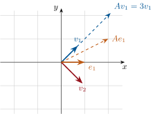
$\lambda \in K$ is an eigenvalue of $u$ when $u(x) = \lambda x$ for some $x \neq 0$ (an eigenvector); the eigenspace is $E_\lambda(u) = \ker(u - \lambda\,\mathrm{id})$ . The set of eigenvalues is the spectrum $\operatorname{Sp}(u)$ . A subspace $F$ is stable when $u(F) \subseteq F$ ; eigenspaces are stable, and stable subspaces allow induced endomorphisms $u|_F$ .

Theorem 3.2 (Independence of eigenspaces)

Eigenvectors associated with pairwise distinct eigenvalues form a free family; equivalently, the sum of the eigenspaces $E_{\lambda_1} + \dots + E_{\lambda_r}$ (distinct $\lambda_i$ ) is direct. In particular $u$ has at most $n$ eigenvalues.

Proof. By induction on $r$ . Suppose $x_1 + \dots + x_r = 0$ with $x_i \in E_{\lambda_i}$ , the statement known for $r - 1$ . Apply $u$ and subtract $\lambda_r$ times the relation:

\sum_{i=1}^{r-1} (\lambda_i - \lambda_r)\, x_i = 0 ,

so by induction each $(\lambda_i - \lambda_r)x_i = 0$ , i.e. $x_i = 0$ for $i < r$ , then $x_r = 0$ . Direct sums of nonzero spaces in a space of dimension $n$ have at most $n$ summands. ∎

The matrix A = psmallmatrix2 & 1\\ 1 & 2 psmallmatrix acting on the plane: the generic vector e_1 is knocked off its line, but the eigendirections v_1 = (1,1) and v_2 = (1,-1) are merely stretched — by 3 and by 1 (so Av_2 = v_2: the dashed image coincides with v_2). Diagonalization is the change to the basis (v_1, v_2), where A becomes diag(3, 1). — The matrix $A = \left(\begin{smallmatrix}2 & 1\\ 1 & 2\end{smallmatrix}\right)$ acting on the plane: the generic vector $e_1$ is knocked off its line, but the eigendirections $v_1 = (1,1)$ and $v_2 = (1,-1)$ are merely stretched — by $3$ and by $1$ (so $Av_2 = v_2$ : the dashed image coincides with $v_2$ ). Diagonalization is the change to the basis $(v_1, v_2)$ , where $A$ becomes $\operatorname{diag}(3, 1)$ .

Definition 3.3 (Characteristic polynomial)

$\chi_u(X) = \det(X\,\mathrm{id} - u)$ — computed in any basis as $\det(XI_n - A)$ , a monic polynomial of degree $n$ , invariant under similarity (Theorem 2.17). Its roots in $K$ are exactly the eigenvalues ( $\lambda$ eigenvalue $\iff u - \lambda\,\mathrm{id}$ not injective $\iff \chi_u(\lambda) = 0$ ), and

\chi_u(X) = X^n - (\operatorname{tr} u)\, X^{n-1} + \dots + (-1)^n \det u .

The algebraic multiplicity $m_\lambda$ of an eigenvalue is its multiplicity as a root of $\chi_u$ ; the geometric multiplicity is $\dim E_\lambda$ , and $1 \leq \dim E_\lambda \leq m_\lambda$ .

Proof of the stated facts. The coefficient claims: expand $\det(XI - A)$ by the permutation formula; the identity permutation contributes $\prod_i (X - a_{ii}) = X^n - (\sum a_{ii})X^{n-1} + \dots$ , and every other permutation fixes at most $n - 2$ diagonal positions, contributing degree $\leq n - 2$ : the top two coefficients are as stated; $X = 0$ gives the constant term $\det(-A) = (-1)^n\det A$ .

Geometric $\leq$ algebraic: let $d = \dim E_\lambda$ and complete a basis of $E_\lambda$ into a basis of $E$ ; the matrix of $u$ is block upper-triangular with top-left block $\lambda I_d$ , so $\chi_u(X) = (X - \lambda)^d\, \chi_{\text{(bottom block)}}(X)$ : the multiplicity of $\lambda$ is at least $d$ . ∎

Example 3.4 (Same $\chi$ , different geometry)

The matrices

\begin{pmatrix}2 & 0\\ 0 & 2\end{pmatrix} \qquad\text{and}\qquad \begin{pmatrix}2 & 1\\ 0 & 2\end{pmatrix}

share the characteristic polynomial $(X - 2)^2$ , the trace, the determinant, the spectrum — yet are not similar: the first has $E_2$ of dimension $2$ (geometric multiplicity $2$ ), the second of dimension $1$ . The characteristic polynomial sees only algebraic multiplicities; the eigenspace dimensions are the finer invariant, and the minimal polynomial arbitrates ( $X - 2$ versus $(X - 2)^2$ ). Moral for all diagonalizability discussions: $\chi$ shortlists the candidates, but kernels cast the votes.

Definition 3.5 (Diagonalizable, trigonalizable)

$u$ is diagonalizable when $E$ has a basis of eigenvectors (matrix: similar to a diagonal matrix); trigonalizable when its matrix in some basis is upper triangular.

Theorem 3.6 (Diagonalizability criteria)

The following are equivalent:

$u$ is diagonalizable;
$E = \bigoplus_{\lambda \in \operatorname{Sp} u} E_\lambda$ ;
$\chi_u$ splits over $K$ and $\dim E_\lambda = m_\lambda$ for every eigenvalue;
(sufficient, not necessary) $\chi_u$ has $n$ distinct roots in $K$ .

Proof. (1 $\iff$ 2): a basis of eigenvectors sorts into bases of the $E_\lambda$ ’s, and conversely concatenating bases of the direct summands gives a basis of $E$ (Theorem 3.2 makes the sum direct; equality of dimensions makes it everything).

(2 $\iff$ 3): in the diagonal basis, $\chi_u = \prod (X - \lambda)^{\dim E_\lambda}$ splits with matching multiplicities. Conversely, suppose $\chi_u$ splits with $\dim E_\lambda = m_\lambda$ throughout; then the direct sum of the eigenspaces (direct by Theorem 3.2) has dimension

\sum_{\lambda}\dim E_\lambda = \sum_{\lambda} m_\lambda = \deg\chi_u = n ,

the middle equality because a split polynomial’s degree is the sum of its root multiplicities: the sum is all of $E$ . Note where each hypothesis worked: splitting filled the degree, equality of multiplicities filled the dimensions.

(4 $\Rightarrow$ 1): $n$ distinct eigenvalues give $n$ independent eigenvectors (Theorem 3.2): a basis. ∎

Method 3.7 (Deciding diagonalizability)

In practice, test in this order — each step may finish the job. (1) Does an annihilating polynomial with simple split roots present itself ( $u^2 = \mathrm{id}$ , $u^2 = u$ , $u^k = \mathrm{id}$ )? If yes: diagonalizable, no computation (Corollary 3.17 below). (2) Compute $\chi_u$ ; if it has $n$ distinct roots in $K$ : diagonalizable (Theorem 3.6 (4)). (3) Otherwise, for each multiple root $\lambda$ only, compare $\dim\ker(u - \lambda\,\mathrm{id})$ with the multiplicity $m_\lambda$ : any deficit kills diagonalizability; equality everywhere proves it. Never compute eigenspaces of simple roots (their dimension is forced to be $1$ ), and never trigonalize just to decide.

Example 3.8 (Diagonalization put to work)

$A = I + J = \left(\begin{smallmatrix}2 & 1 & 1\\ 1 & 2 & 1\\ 1 & 1 & 2\end{smallmatrix}\right)$ , with $J$ the all-ones matrix: from $\operatorname{Sp}(J) = \{3, 0\}$ (Example 2.19), $\operatorname{Sp}(A) = \{4, 1\}$ , with eigenspaces $\R(1,1,1)$ and the plane $\{x + y + z = 0\}$ : dimensions $1 + 2 = 3$ , diagonalizable (Theorem 3.6 (2)). Powers without any change-of-basis matrix: with $\Pi = J/3$ the projector onto $\R(1,1,1)$ ,

A = 4\,\Pi + 1\cdot(I - \Pi) \quad\Longrightarrow\quad A^k = 4^k\,\Pi + (I - \Pi) = \frac{4^k - 1}{3}\,J + I .

(Check $k = 1$ : $\frac{4-1}3 J + I = A$ .) The closing insight: when the eigenspaces are visible, spectral projectors compute powers faster than $PDP^{-1}$ ever will — and the formula displays the dynamics: $A^k$ grows like $4^k$ along $(1,1,1)$ and stays put on the orthogonal plane.

Theorem 3.9 (Trigonalization)

$u$ is trigonalizable over $K$ if and only if $\chi_u$ splits over $K$ . In particular every endomorphism of a $\C$ -vector space is trigonalizable.

Proof. ( $\Rightarrow$ ) The characteristic polynomial of a triangular matrix is $\prod(X - t_{ii})$ : split.

( $\Leftarrow$ ) Induction on $n$ . Since $\chi_u$ splits, it has a root $\lambda$ : pick an eigenvector $e_1$ . In a basis starting with $e_1$ , the matrix is $\begin{pmatrix} \lambda & \ast\\ 0 & B\end{pmatrix}$ , and $\chi_u = (X - \lambda)\chi_B$ : $\chi_B$ splits too. By the induction hypothesis applied to the $(n-1) \times (n-1)$ matrix $B$ , there is an invertible $Q$ with $Q^{-1}BQ$ upper triangular; conjugating the whole matrix by $\begin{pmatrix}1 & 0\\ 0 & Q\end{pmatrix}$ triangularizes it. ∎

Example 3.10 (Trigonalizing by hand)

$B = \begin{pmatrix}3 & -1\\ 1 & 1\end{pmatrix}$ : $\chi_B = X^2 - 4X + 4 = (X - 2)^2$ , and $\ker(B - 2I) = \ker\left(\begin{smallmatrix}1 & -1\\ 1 & -1\end{smallmatrix}\right)$ is the line spanned by $e_1' = (1, 1)$ : one eigenvalue, a one-dimensional eigenspace — not diagonalizable, but trigonalizable (Theorem 3.9). Complete the basis with $e_2' = (1, 0)$ and compute:

u(e_1') = (2, 2) = 2e_1', \qquad u(e_2') = (3, 1) = 1\cdot e_1' + 2\, e_2' ,

so in the basis $(e_1', e_2')$ the matrix is $T = \left(\begin{smallmatrix}2 & 1\\ 0 & 2\end{smallmatrix}\right)$ . The closing insight: the diagonal of $T$ was forced (both entries must be the double eigenvalue $2$ ); only the corner entry depended on the choice of $e_2'$ , and rescaling $e_2'$ can make it any nonzero value — the resistant “ $1$ ” is the shadow of the nilpotent part that Dunford will isolate.

3.2 Polynomials of an endomorphism

Definition 3.11

For $P = \sum a_k X^k \in K[X]$ , set $P(u) = \sum a_k u^k \in \mathcal{L}(E)$ . The map $P \mapsto P(u)$ is a morphism of algebras $K[X] \to \mathcal{L}(E)$ (Definition 1.33); its kernel $\{P : P(u) = 0\}$ is an ideal of $K[X]$ , nonzero (the family $(\mathrm{id}, u, \dots, u^{n^2})$ is linked in the $n^2$ -dimensional $\mathcal{L}(E)$ ), hence generated by a unique monic polynomial $\mu_u$ : the minimal polynomial (Theorem 1.26).

Proposition 3.12

$P(u) = 0 \iff \mu_u \mid P$ ; eigenvalues of $u$ are roots of every annihilating polynomial, and the roots of $\mu_u$ are exactly the eigenvalues.
If $F$ is stable, $\mu_{u|_F} \mid \mu_u$ .

Proof. (1) The divisibility is the definition of a generator. If $u(x) = \lambda x$ , $x \neq 0$ , then $0 = P(u)(x) = P(\lambda)x$ , so $P(\lambda) = 0$ : eigenvalues are roots of annihilators, in particular of $\mu_u$ . Conversely, if $\lambda$ is a root, $\mu_u = (X - \lambda)Q$ with $Q(u) \neq 0$ (degree of $\mu_u$ minimal): pick $y$ with $Q(u)(y) \neq 0$ ; then $(u - \lambda)(Q(u)(y)) = \mu_u(u)(y) = 0$ exhibits the eigenvector $Q(u)(y)$ .

(2) $\mu_u(u|_F) = \mu_u(u)|_F = 0$ , and apply (1) to $u|_F$ . ∎

Example 3.13 (Minimal polynomials found by hand)

The minimal polynomial is computed by testing successive degrees. For the all-ones matrix $J \in \mathcal{M}_3(\R)$ : $J \neq \lambda I$ (degree $1$ is out), and $J^2 = 3J$ , so

\mu_J = X^2 - 3X = X(X - 3) :

degree $2$ , split, simple roots — $J$ is diagonalizable with spectrum $\{0, 3\}$ (Corollary 3.17 below), confirming Example 2.19 without a single determinant. For the swap matrix $A$ of Example 3.15: $A \neq \pm I$ and $A^2 = I$ give $\mu_A = X^2 - 1$ . In both cases the pattern is the same: guess a low-degree identity from the structure (rank one forces $J^2 = (\operatorname{tr}J)\,J$ ; an involution forces $A^2 = I$ ), then check that no proper divisor annihilates. Minimal polynomials are usually found, not computed from $\chi$ .

Theorem 3.14 (Kernel decomposition lemma)

If $P = P_1 P_2 \cdots P_r$ with the $P_i$ pairwise coprime, then

\ker P(u) = \ker P_1(u) \oplus \dots \oplus \ker P_r(u),

and the projections onto the summands are polynomials in $u$ .

Proof. It suffices to treat $r = 2$ and induct. Bézout in $K[X]$ (Theorem 1.26): $U P_1 + V P_2 = 1$ , so for every $x$ ,

x = \underbrace{U(u)P_1(u)(x)}_{=:\,x_2} + \underbrace{V(u)P_2(u)(x)}_{=:\,x_1}.

If $x \in \ker P(u)$ : $P_2(u)(x_2) = U(u)\,P(u)(x) = 0$ (polynomials in $u$ commute), so $x_2 \in \ker P_2(u)$ , and symmetrically $x_1 \in \ker P_1(u)$ : the sum fills $\ker P(u)$ ; both summands sit inside $\ker P(u)$ ( $P_i \mid P$ ). Directness: $x \in \ker P_1(u) \cap \ker P_2(u)$ gives $x = U(u)P_1(u)x + V(u)P_2(u)x = 0$ . The formulas for $x_1, x_2$ exhibit the projections as $V(u)P_2(u)$ and $U(u)P_1(u)$ . ∎

Example 3.15 (The kernel lemma with explicit projectors)

Let $A = \left(\begin{smallmatrix}0 & 1 & 0\\ 1 & 0 & 0\\ 0 & 0 & 1\end{smallmatrix}\right)$ (swap the first two coordinates). Then $A^2 = I$ : the polynomial $X^2 - 1 = (X - 1)(X + 1)$ annihilates $A$ , its factors are coprime, and Bézout is explicit:

\frac{1}{2}(X + 1) - \frac12(X - 1) = 1 .

Following the proof of Theorem 3.14, the projections onto $\ker(A - I)$ and $\ker(A + I)$ are the polynomials in $A$

\pi_+ = \frac{A + I}{2} = \frac12\begin{pmatrix} 1 & 1 & 0\\ 1 & 1 & 0\\ 0 & 0 & 2\end{pmatrix}, \qquad \pi_- = \frac{I - A}{2} = \frac12\begin{pmatrix} 1 & -1 & 0\\ -1 & 1 & 0\\ 0 & 0 & 0\end{pmatrix}.

Check: $\pi_+ + \pi_- = I$ , $\pi_+\pi_- = 0$ , $\pi_\pm^2 = \pi_\pm$ , and the images are the plane $\{x = y\}$ (symmetric vectors, eigenvalue $1$ ) and the line $\R(1, -1, 0)$ (antisymmetric, eigenvalue $-1$ ). The kernel lemma is not an existence statement: Bézout coefficients are the projector formulas.

Example 3.16 (Projectors compute the exponential too)

The same swap matrix, one dividend further. Since $A = \pi_+ - \pi_-$ with orthogonal-in-the-algebraic-sense projectors ( $\pi_+\pi_- = 0$ ), every power obeys $A^k = \pi_+ + (-1)^k\pi_-$ , and the exponential series regroups by projector:

\eu^{tA} = \sum_k \frac{t^k}{k!}\bigl(\pi_+ + (-1)^k\pi_-\bigr) = \eu^{t}\,\pi_+ + \eu^{-t}\,\pi_- = \begin{pmatrix} \cosh t & \sinh t & 0\\ \sinh t & \cosh t & 0\\ 0 & 0 & \eu^{t} \end{pmatrix}.

(Check $t = 0$ : the identity; derivative at $0$ : $A$ .) The eigendecomposition converts a matrix series into two scalar series — the exact mechanism that Chapter 16 will run on every diagonalizable system, and the reason hyperbolic functions govern symmetric couplings.

Corollary 3.17 (Diagonalizability via the minimal polynomial)

$u$ is diagonalizable $\iff$ $\mu_u$ splits over $K$ with simple roots $\iff$ some annihilating polynomial of $u$ splits with simple roots.

Proof. If $P(u) = 0$ with $P = \prod_{i}(X - \lambda_i)$ (distinct $\lambda_i$ ), the lemma gives $E = \ker P(u) = \bigoplus_i \ker(u - \lambda_i)$ : a direct sum of eigenspaces, so $u$ is diagonalizable (Theorem 3.6). Conversely, a diagonalizable $u$ is killed by $\prod_{\lambda \in \operatorname{Sp}u}(X - \lambda)$ (it kills each eigenspace), which splits with simple roots; and $\mu_u$ divides it while having the same roots (Proposition 3.12): $\mu_u$ is exactly that product. ∎

Example 3.18

Projections satisfy $p^2 = p$ : annihilated by $X(X-1)$ , split simple roots — diagonalizable with spectrum $\subseteq \{0, 1\}$ , and $E = \ker p \oplus \ker(p - \mathrm{id})$ : Year 1’s geometric analysis, re-proved in one line. Symmetries ( $s^2 = \mathrm{id}$ , annihilator $X^2 - 1$ ): diagonalizable when $\operatorname{char} K \neq 2$ , spectrum $\subseteq \{\pm 1\}$ . An endomorphism with $u^3 = u^2$ and $u^2 \neq u$ : annihilated by $X^2(X - 1)$ , not necessarily diagonalizable — the criterion detects it (double root $0$ must be tested: diagonalizable iff moreover $\ker u^2 = \ker u$ ).

Example 3.19 (The field decides: a rotation in $\R^3$ )

Let $R$ be the quarter-turn around the $z$ -axis:

R = \begin{pmatrix} 0 & -1 & 0\\ 1 & 0 & 0\\ 0 & 0 & 1 \end{pmatrix}, \qquad \chi_R = (X - 1)(X^2 + 1).

Over $\R$ : the only eigenvalue is $1$ , with eigenspace the axis $\R e_3$ — one line of fixed vectors, and no further reduction: $R$ is neither diagonalizable nor trigonalizable in $\mathcal{M}_3(\R)$ ( $\chi_R$ does not split). Over $\C$ : three distinct eigenvalues $1, \iu, -\iu$ , so $R$ is diagonalizable, with eigenvectors $e_3$ and $e_1 \mp \iu e_2$ . The geometry was audible in the algebra: rotations in the plane have no real invariant directions, and the complex eigenvalues $\pm\iu$ of modulus $1$ store the angle ( $\pm\frac\pi2$ ) that the real matrix can only express by mixing coordinates.

Example 3.20 (Minimal versus characteristic)

For $D = \operatorname{diag}(2, 2, 3)$ : $\chi_D = (X - 2)^2(X - 3)$ but $\mu_D = (X - 2)(X - 3)$ , since $(D - 2I)(D - 3I) = 0$ (check on the canonical basis) while neither factor alone kills $D$ . For the shift block $N = \left(\begin{smallmatrix}0 & 1\\ 0 & 0\end{smallmatrix}\right) \oplus (3)$ , i.e. $N' = \left(\begin{smallmatrix}0 & 1 & 0\\ 0 & 0 & 0\\ 0 & 0 & 3\end{smallmatrix}\right)$ : $\chi_{N'} = X^2(X - 3)$ and $\mu_{N'} = X^2(X - 3)$ — the double root is genuinely needed because $N'$ is not diagonalizable on $\ker$ -side ( $N'e_2 = e_1 \neq 0$ ). Rule of thumb: $\mu$ and $\chi$ share their roots (Proposition 3.12); the multiplicity in $\mu$ measures the size of the largest nilpotent block, the one in $\chi$ the total dimension of the characteristic subspace.

Theorem 3.21 (Cayley–Hamilton)

$\chi_u(u) = 0$ ; consequently $\mu_u \mid \chi_u$ , and $\deg \mu_u \leq n$ .

Proof. Fix $x \neq 0$ and let $d$ be maximal with $(x, u(x), \dots, u^{d-1}(x))$ free; write

u^d(x) = -a_0 x - a_1 u(x) - \dots - a_{d-1}u^{d-1}(x),

and set $P_x = X^d + a_{d-1}X^{d-1} + \dots + a_0$ , so $P_x(u)(x) = 0$ . Complete the free family into a basis of $E$ : on it, $u$ has block form $\begin{pmatrix} C & \ast\\ 0 & D\end{pmatrix}$ where $C$ is the companion matrix of $P_x$ , whose characteristic polynomial is $P_x$ (expand $\det(XI - C)$ along the first column, by induction on $d$ ). Hence $\chi_u = P_x \cdot \chi_D$ , and

\chi_u(u)(x) = \chi_D(u)\bigl(P_x(u)(x)\bigr) = 0 .

The argument holds for every $x$ : $\chi_u(u) = 0$ . ∎

Example 3.22 (Cayley–Hamilton at work)

$A = \begin{pmatrix} 1 & 2\\ 3 & 4\end{pmatrix}$ : $\chi_A = X^2 - 5X - 2$ , so $A^2 = 5A + 2I$ . Every power of $A$ collapses to a combination of $I$ and $A$ :

A^4 = (5A + 2I)^2 = 25A^2 + 20A + 4I = 145A + 54I = \begin{pmatrix} 199 & 290\\ 435 & 634\end{pmatrix},

and the inverse comes free: $A(A - 5I) = 2I$ gives

A^{-1} = \tfrac12(A - 5I) = \begin{pmatrix} -2 & 1\\ 3/2 & -1/2\end{pmatrix}.

The closing insight: Cayley–Hamilton compresses the whole algebra $K[A]$ into $\operatorname{Vect}(I, A, \dots, A^{n-1})$ — $\dim K[A] = \deg\mu_A \leq n$ , however large the powers you need.

Remark 3.23 (Common pitfalls)

(i) Eigenvalues do not add: $\operatorname{Sp}(A + B)$ is not $\operatorname{Sp}A + \operatorname{Sp}B$ , and a sum of diagonalizable matrices need not be diagonalizable — $\left(\begin{smallmatrix}1 & 1\\ 0 & 0\end{smallmatrix}\right) + \left(\begin{smallmatrix}0 & 0\\ 0 & 1\end{smallmatrix}\right) = \left(\begin{smallmatrix}1 & 1\\ 0 & 1\end{smallmatrix}\right)$ is a sum of two diagonalizable matrices (each has distinct eigenvalues) and is not diagonalizable; only commuting families behave (Exercise 3.9). (ii) “ $\chi_u$ splits” is a hypothesis about the field: a plane rotation has $\chi = X^2 - 2\cos\theta\,X + 1$ , split over $\C$ , not over $\R$ — diagonalizable in $\mathcal{M}_2(\C)$ , not trigonalizable in $\mathcal{M}_2(\R)$ . (iii) The inequality runs geometric $\leq$ algebraic, never the reverse; testing only $\dim E_\lambda \geq 1$ proves nothing about diagonalizability. (iv) $\mu_u$ is not $\chi_u$ : equality holds exactly when each eigenvalue has a single block chain (e.g. companion matrices, this chapter’s weekend problem); using $\chi$ where $\mu$ is needed inflates every power computation. (v) Dunford’s $d$ and $\nu$ are polynomials in $u$ — a decomposition $u = d' + \nu'$ with the right properties but $d'\nu' \neq \nu'd'$ is not Dunford and is never unique.

Remark 3.24 (Where this chapter is used)

Reduction is the workhorse of the rest of the book: powers and exponentials of matrices drive the linear differential systems of Chapter 16; the spectral theorem of Chapter 12 is diagonalization made orthogonal; generating functions (Chapter 23) re-derive the recurrence asymptotics of this chapter’s weekend problem analytically. In the Year 3 volume the same program runs in infinite dimension: the spectral theory of compact self-adjoint operators, where eigenvalue sequences replace finite spectra, and the Perron–Frobenius theory of positive matrices, which explains why dominant eigenvalues of counting problems are positive and simple.

3.3 Nilpotents and the Dunford decomposition

Proposition 3.25 (Nilpotent endomorphisms)

For $u$ with $\chi_u$ split, the following are equivalent: $u^n = 0$ ; $u^k = 0$ for some $k$ ; $\operatorname{Sp}(u) = \{0\}$ ; $\chi_u = X^n$ ; $u$ is trigonalizable with zero diagonal. A nilpotent endomorphism has $\mu_u = X^{\text{(nilpotence index)}}$ , and index $\leq n$ .

Proof. $u^k = 0$ makes every eigenvalue a root of $X^k$ : spectrum $\{0\}$ (nonempty when $\chi$ splits — over $\C$ always). Then $\chi_u = X^n$ (all roots zero) and Cayley–Hamilton gives $u^n = 0$ ; trigonalization (Theorem 3.9) puts zeros on the diagonal (the diagonal carries the eigenvalues). Conversely, let $A$ be strictly upper triangular: $a_{ij} = 0$ for $j \leq i$ . We show by induction that

(A^k)_{ij} = 0 \qquad \text{whenever } j \leq i + k - 1,

i.e. each power pushes the zero region one diagonal higher. For $k = 1$ this is the hypothesis. For the step,

(A^{k+1})_{ij} = \sum_{\ell} (A^k)_{i\ell}\,a_{\ell j} ,

and each term vanishes: either $\ell \leq i + k - 1$ (the first factor is $0$ by induction) or $\ell \geq i + k$ , in which case $j \leq i + k \leq \ell$ kills the second factor. At $k = n$ the condition $j \leq i + n - 1$ holds for all $i, j \leq n$ : $A^n = 0$ . The minimal polynomial divides $X^n$ and annihilation defines the index. ∎

Theorem 3.26 (Dunford decomposition)

Suppose $\chi_u$ splits over $K$ (automatic for $K = \C$ ). Then there is a unique pair $(d, \nu)$ with

u = d + \nu, \qquad d \text{ diagonalizable}, \quad \nu \text{ nilpotent}, \quad d\nu = \nu d ,

and moreover $d$ and $\nu$ are polynomials in $u$ .

Proof. Existence. Write $\chi_u = \prod_{i=1}^{r} (X - \lambda_i)^{m_i}$ (distinct $\lambda_i$ ) and set $N_i = \ker(u - \lambda_i)^{m_i}$ , the characteristic subspaces. By Cayley–Hamilton and the kernel lemma (Theorem 3.14),

E = N_1 \oplus \dots \oplus N_r ,

with projections $\pi_i$ polynomial in $u$ ; each $N_i$ is stable (polynomials in $u$ commute with $u$ ). Define $d = \sum_i \lambda_i \pi_i$ : a polynomial in $u$ , diagonalizable (it acts as $\lambda_i$ on $N_i$ , so $E$ decomposes into its eigenspaces). Then $\nu = u - d$ is a polynomial in $u$ (hence commutes with $d$ ), and on each $N_i$ it acts as $u - \lambda_i$ , with $(u - \lambda_i)^{m_i} = 0$ there: $\nu^{\max m_i} = 0$ on each summand, so $\nu$ is nilpotent.

Uniqueness. Let $u = d' + \nu'$ be another such pair. Since $d'$ and $\nu'$ commute with each other, they commute with $u = d' + \nu'$ , hence with every polynomial in $u$ — in particular with $d$ and $\nu$ . Then $d - d'$ is diagonalizable (two commuting diagonalizable maps are simultaneously diagonalizable: Exercise 3.9) and equals $\nu' - \nu$ , which is nilpotent: if $\nu^k = 0$ and $\nu'^{k'} = 0$ , commutation licenses the binomial expansion

(\nu' - \nu)^{k + k' - 1} = \sum_{j=0}^{k+k'-1}\binom{k + k' - 1}{j} \,\nu'^{\,j}\,(-\nu)^{k + k' - 1 - j} ,

in which every term dies: either $j \geq k'$ (first factor zero) or $k + k' - 1 - j \geq k$ (second factor zero), and one of the two always holds. A diagonalizable nilpotent is zero (its spectrum is $\{0\}$ and it is diagonal in some basis): $d = d'$ , $\nu = \nu'$ . ∎

Example 3.27 (Powers and exponentials)

$A = \begin{pmatrix} 3 & 1\\ -1 & 1\end{pmatrix}$ : $\chi_A = X^2 - 4X + 4 = (X-2)^2$ , single eigenvalue $2$ , eigenspace of dimension $1$ : not diagonalizable. Dunford: $D = 2I$ , $N = A - 2I = \begin{pmatrix} 1 & 1\\ -1 & -1\end{pmatrix}$ , $N^2 = 0$ . Then

A^k = (2I + N)^k = 2^k I + k\,2^{k-1} N , \qquad \eu^{tA} = \eu^{2t}(I + tN),

by the commuting binomial theorem, resp. the exponential series (Chapter 16) split on commuting summands. Reduction turns matrix dynamics into scalar dynamics.

Remark 3.28 (Perspectives within this volume)

Reduction is a hub; here are the four spokes to watch. In Chapter 5, adapted norms turn “all eigenvalues of modulus $< 1$ ” into “some operator norm $< 1$ ”, making spectra govern convergence of powers and series. In Chapter 16, the recipe of Example 3.27 becomes the general solution of $X' = AX$ : Dunford splits $\eu^{tA}$ into polynomial-times-exponential blocks, and stability reads off the real parts of eigenvalues. In Chapter 12, a scalar product forces what mere linear algebra cannot: symmetric matrices become orthogonally diagonalizable, with no nilpotent part at all. And in Chapter 23, the dominant-eigenvalue asymptotics of this chapter’s weekend problem reappear analytically, as the smallest singularity of a generating function — two languages for one growth rate.

3.4 Exercises

Exercise 3.1 ★

Diagonalize (eigenvalues, bases of eigenspaces, invertible $P$ ):

A = \begin{pmatrix} 1 & 2\\ 2 & 1 \end{pmatrix}, \qquad B = \begin{pmatrix} 0 & 1 & 1\\ 1 & 0 & 1\\ 1 & 1 & 0 \end{pmatrix}.

Solution

Solution of Exercise 3.1.

$A$ : $\chi_A = X^2 - 2X - 3 = (X - 3)(X + 1)$ . Eigenvectors: for $3$ : $(1,1)$ ; for $-1$ : $(1,-1)$ . So $P = \begin{pmatrix} 1 & 1\\ 1 & -1\end{pmatrix}$ gives $P^{-1}AP = \operatorname{diag}(3, -1)$ .

$B = J - I$ where $J$ is the all-ones matrix. $J$ has rank $1$ with $Jv = 3v$ for $v = (1,1,1)$ and $Jw = 0$ on the plane $x + y + z = 0$ : spectrum of $B$ is $\{2, -1\}$ with eigenspaces $\operatorname{Vect}(1,1,1)$ (dimension $1$ ) and $\{x + y + z = 0\}$ (dimension $2$ , basis $(1,-1,0), (1,0,-1)$ ). $P$ with these three columns gives $P^{-1}BP = \operatorname{diag}(2, -1, -1)$ .

Exercise 3.2 ★

Show that $C = \begin{pmatrix} 1 & 1\\ 0 & 1\end{pmatrix}$ is not diagonalizable, twice: via eigenspaces, and via the minimal polynomial.

Solution

Solution of Exercise 3.2.

Eigenspaces: $\chi_C = (X-1)^2$ , single eigenvalue $1$ ; $\ker(C - I) = \ker\begin{pmatrix} 0&1\\ 0&0\end{pmatrix}$ is the line $\operatorname{Vect}(e_1)$ : dimension $1 < 2 = m_1$ , so not diagonalizable (Theorem 3.6).

Minimal polynomial: $\mu_C$ divides $(X-1)^2$ and $C \neq I$ , so $\mu_C = (X-1)^2$ : a double root, so not diagonalizable (Corollary 3.17).

Exercise 3.3 ★

Let $u$ satisfy $u^2 - 5u + 6\,\mathrm{id} = 0$ . Prove that $u$ is diagonalizable, determine the possible spectra, and compute $u^k$ as a combination of $\mathrm{id}$ and $u$ .

Solution

Solution of Exercise 3.3.

$X^2 - 5X + 6 = (X-2)(X-3)$ : split with simple roots, so $u$ is diagonalizable (Corollary 3.17), with $\operatorname{Sp}(u) \subseteq \{2, 3\}$ . Possible spectra: $\{2\}$ ( $u = 2\,\mathrm{id}$ ), $\{3\}$ ( $u = 3\,\mathrm{id}$ ), or $\{2, 3\}$ .

Powers: seek $u^k = a_k\,\mathrm{id} + b_k\,u$ . On the eigenspaces, this reads $2^k = a_k + 2b_k$ and $3^k = a_k + 3b_k$ : solving, $b_k = 3^k - 2^k$ , $a_k = 3\cdot2^k - 2\cdot 3^k$ :

u^k = (3\cdot 2^k - 2\cdot 3^k)\,\mathrm{id} + (3^k - 2^k)\, u .

(Valid for all three spectra: the identities hold eigenvalue-wise.)

Exercise 3.4 ★★

Let $u$ be diagonalizable and $F$ a stable subspace. Prove that $u|_F$ is diagonalizable (restrict an annihilating polynomial with simple split roots).

Solution

Solution of Exercise 3.4.

$u$ diagonalizable: $P = \prod_{\lambda}(X - \lambda)$ over the spectrum annihilates $u$ , splits, simple roots. Then $P(u|_F) = P(u)|_F = 0$ : the restriction is annihilated by a split polynomial with simple roots, hence diagonalizable (Corollary 3.17).

Exercise 3.5 ★★

(Fibonacci) Let $A = \begin{pmatrix} 1 & 1\\ 1 & 0\end{pmatrix}$ . Diagonalize $A$ over $\R$ , and deduce Binet’s formula for the Fibonacci sequence ( $F_0 = 0$ , $F_1 = 1$ , $F_{n+1} = F_n + F_{n-1}$ ):

F_n = \frac{\varphi^n - \psi^n}{\sqrt 5}, \qquad \varphi = \frac{1 + \sqrt5}{2},\ \psi = \frac{1 - \sqrt5}{2}.

Solution

Solution of Exercise 3.5.

$\chi_A = X^2 - X - 1$ , roots $\varphi$ and $\psi$ (distinct): diagonalizable, with eigenvectors $(\varphi, 1)$ and $(\psi, 1)$ . The recurrence gives $\begin{pmatrix} F_{n+1}\\ F_n \end{pmatrix} = A^n \begin{pmatrix}1\\ 0\end{pmatrix}$ . Decompose $(1, 0)$ on the eigenvectors: $(1,0) = \frac{1}{\varphi - \psi}\bigl((\varphi, 1) - (\psi, 1)\bigr)$ with $\varphi - \psi = \sqrt5$ . Applying $A^n$ multiplies each eigencomponent by its eigenvalue’s $n$ -th power; reading the second coordinate:

F_n = \frac{\varphi^n - \psi^n}{\sqrt 5} .

(Check: $n = 1$ gives $\frac{\varphi - \psi}{\sqrt5} = 1$ .)

Exercise 3.6 ★★

Let $u \in \mathcal{L}(E)$ with $u^2$ diagonalizable and $u$ invertible ( $K = \C$ ). Prove that $u$ is diagonalizable. Give a counterexample when $u$ is not invertible.

Solution

Solution of Exercise 3.6.

Let $P = \prod_i (X - \mu_i)$ annihilate $u^2$ , split with simple roots $\mu_i$ (the spectrum of $u^2$ ). Since $u$ is invertible, $0$ is not an eigenvalue of $u^2$ ( $\det u^2 = (\det u)^2 \neq 0$ ), so all $\mu_i \neq 0$ . Then

Q(X) = \prod_i (X^2 - \mu_i) = \prod_i (X - \sqrt{\mu_i})(X + \sqrt{\mu_i})

annihilates $u$ : $\;Q(u) = \prod_i (u^2 - \mu_i\,\mathrm{id}) = P(u^2) = 0$ . Its roots $\pm \sqrt{\mu_i}$ (complex square roots) are pairwise distinct because the $\mu_i$ are distinct and nonzero ( $\sqrt{\mu_i} = -\sqrt{\mu_j}$ would give $\mu_i = \mu_j$ ). Split + simple roots: $u$ is diagonalizable.

Counterexample without invertibility: $u = \begin{pmatrix} 0 & 1\\ 0 & 0\end{pmatrix}$ : $u^2 = 0$ is diagonalizable, $u$ is not.

Exercise 3.7 ★★

Compute the Dunford decomposition, $A^k$ , and $\eu^{tA}$ for

A = \begin{pmatrix} 2 & 1 & 0\\ 0 & 2 & 1\\ 0 & 0 & 2 \end{pmatrix}.

Solution

Solution of Exercise 3.7.

$A = 2I + N$ with $N$ the shift ( $N e_2 = e_1$ , $Ne_3 = e_2$ ), $N^3 = 0$ , $N^2 = E_{13}$ : this is the Dunford decomposition ( $2I$ diagonal, $N$ nilpotent, they commute; uniqueness makes it the one). Binomial with commuting terms:

A^k = 2^k I + k 2^{k-1} N + \binom k2 2^{k-2} N^2 = \begin{pmatrix} 2^k & k2^{k-1} & \binom k2 2^{k-2}\\ 0 & 2^k & k2^{k-1}\\ 0 & 0 & 2^k \end{pmatrix},

\eu^{tA} = \eu^{2t}\Bigl(I + tN + \frac{t^2}{2}N^2\Bigr) = \eu^{2t}\begin{pmatrix} 1 & t & t^2/2\\ 0 & 1 & t\\ 0 & 0 & 1 \end{pmatrix}.

Exercise 3.8 ★★

Let $A \in \mathcal{M}_n(\C)$ with $A^k = I$ for some $k \geq 1$ . Prove that $A$ is diagonalizable and its eigenvalues are $k$ -th roots of unity. Deduce that a finite-order invertible complex matrix similar to a triangular matrix with unit diagonal is the identity.

Solution

Solution of Exercise 3.8.

$X^k - 1$ annihilates $A$ and splits over $\C$ with the $k$ distinct roots $\eu^{2\iu\pi j/k}$ : $A$ is diagonalizable (Corollary 3.17) and its eigenvalues, roots of $X^k - 1$ , are $k$ -th roots of unity.

If moreover $A$ is similar to a triangular matrix with unit diagonal: all eigenvalues equal $1$ , and $A$ , diagonalizable with sole eigenvalue $1$ , is $P\,I\,P^{-1} = I$ .

Exercise 3.9 ★★★

(Simultaneous diagonalization) Let $u, v$ be diagonalizable and commuting. Prove that they are simultaneously diagonalizable: some basis diagonalizes both. (Each eigenspace of $u$ is $v$ -stable; diagonalize the restrictions of $v$ there, using Exercise 3.4.)

Solution

Solution of Exercise 3.9.

Write $E = \bigoplus_\lambda E_\lambda(u)$ (Theorem 3.6). Each $E_\lambda(u)$ is $v$ -stable: for $x \in E_\lambda$ , $u(v(x)) = v(u(x)) = \lambda v(x)$ . The restriction of $v$ to $E_\lambda(u)$ is diagonalizable (Exercise 3.4): choose a basis of $E_\lambda(u)$ made of $v$ -eigenvectors. Concatenating these bases over all $\lambda$ gives a basis of $E$ whose vectors are eigenvectors of both $u$ (by membership in $E_\lambda(u)$ ) and $v$ (by construction).

Exercise 3.10 ★★★

Let $u \in \mathcal{L}(\C^n)$ . Prove that $u$ is diagonalizable if and only if every $u$ -stable subspace has a $u$ -stable supplementary subspace. (For $\Leftarrow$ : apply the property to $F = \sum_\lambda E_\lambda(u)$ , the sum of all eigenspaces; if a stable supplement $G$ were nonzero, trigonalizing $u|_G$ would produce an eigenvector of $u$ inside $G$ — contradicting $G \cap F = \{0\}$ .)

Solution

Solution of Exercise 3.10.

( $\Rightarrow$ ) Let $u$ be diagonalizable and $F$ stable. Then $u|_F$ is diagonalizable (Exercise 3.4): $F$ has a basis of eigenvectors, which extends, inside each global eigenspace $E_\lambda$ , to a basis of $E_\lambda$ (incomplete basis theorem within $E_\lambda$ , starting from the part of $F$ ’s basis lying there — note $F = \bigoplus_\lambda (F \cap E_\lambda)$ since $u|_F$ is diagonalizable). The added vectors span a stable supplement (each lies in some $E_\lambda$ , so their span is $u$ -stable).

( $\Leftarrow$ ) Let $F = \sum_\lambda E_\lambda(u)$ (a stable subspace) and $G$ a stable supplement. If $G \neq \{0\}$ : $\chi_{u|_G}$ splits over $\C$ , so $u|_G$ has an eigenvector $x \in G$ (Theorem 3.9 or directly the existence of a root); but every eigenvector of $u$ lies in $F$ , so $x \in F \cap G = \{0\}$ : contradiction. Hence $G = \{0\}$ and $E = F$ : the eigenspaces fill $E$ , i.e. $u$ is diagonalizable.

Exercise 3.11 ★★★

(Spectral radius by Gelfand-lite, $2\times2$ taste of analysis to come) Let $A \in \mathcal{M}_2(\C)$ with both eigenvalues of modulus $< 1$ . Prove that $A^k \to 0$ entrywise as $k \to \infty$ . (Trigonalize: $A = P(T)P^{-1}$ with $T$ upper triangular; compute $T^k$ explicitly — distinguish equal and distinct eigenvalues — and bound.)

Solution

Solution of Exercise 3.11.

Trigonalize: $A = PTP^{-1}$ , $T = \begin{pmatrix} \lambda & c\\ 0 & \mu\end{pmatrix}$ , $\abs\lambda, \abs\mu < 1$ . Then $A^k = PT^kP^{-1}$ , and it suffices that $T^k \to 0$ .

Distinct eigenvalues: induction gives

T^k = \begin{pmatrix} \lambda^k & c\,\dfrac{\lambda^k - \mu^k}{\lambda - \mu}\\[4pt] 0 & \mu^k \end{pmatrix},

and each entry tends to $0$ ( $\abs{\lambda}^k, \abs\mu^k \to 0$ ).

Equal eigenvalues ( $\mu = \lambda$ ): $T = \lambda I + cE_{12}$ and $T^k = \lambda^k I + k\lambda^{k-1}cE_{12}$ ; the entry $k\lambda^{k-1} \to 0$ since $\abs\lambda < 1$ (geometric beats polynomial). In both cases $T^k \to 0$ entrywise, hence $A^k = PT^kP^{-1} \to 0$ (matrix multiplication by fixed $P, P^{-1}$ is continuous in the entries — each entry of the product is a fixed linear combination).

Exercise 3.12 ★★

Let $u \in \mathcal{L}(\C^n)$ with $\operatorname{rk} u = 1$ ( $n \geq 2$ ). Show that $\chi_u = X^{n-1}(X - \operatorname{tr} u)$ , and that $u$ is diagonalizable if and only if $\operatorname{tr} u \neq 0$ . (Recall from Exercise 2.5 that $u^2 = (\operatorname{tr} u)\,u$ .)

Solution

Solution of Exercise 3.12.

$\ker u$ has dimension $n - 1$ (rank–nullity), so $0$ is an eigenvalue of geometric multiplicity $n - 1$ , and $\chi_u$ is divisible by $X^{n-1}$ (Definition 3.3: geometric $\leq$ algebraic). Write $\chi_u = X^{n-1}(X - \alpha)$ ; the coefficient of $X^{n-1}$ being $-\operatorname{tr} u$ , we get $\alpha = \operatorname{tr} u$ : $\chi_u = X^{n-1}(X - \operatorname{tr} u)$ .

If $\operatorname{tr} u \neq 0$ : the eigenvalue $\operatorname{tr} u$ is a root of $\chi_u$ , so it carries an eigenvector; the eigenspaces for $0$ and $\operatorname{tr} u$ have dimensions $n - 1$ and $\geq 1$ , summing to $\geq n$ : they fill $E$ , and $u$ is diagonalizable (Theorem 3.6). If $\operatorname{tr} u = 0$ : by Exercise 2.5, $u^2 = (\operatorname{tr} u)u = 0$ with $u \neq 0$ : $u$ is a nonzero nilpotent, and a diagonalizable nilpotent is zero (Proposition 3.25): not diagonalizable.

3.5 Problem: Linear Recurrences and Companion Matrices

A linear recurrence $u_{n+k} = a_{k-1}u_{n+k-1} + \dots + a_0 u_n$ is a matrix power in disguise, and reduction converts it into closed formulas, growth rates, and error estimates. This weekend problem develops the dictionary — companion matrices on one side, the shift operator on the space of sequences on the other — proves the fundamental theorem of linear recurrences (the general solution is $\sum_i Q_i(n)\lambda_i^n$ over the roots of the characteristic polynomial), and spends the dividends on Diophantine approximation of $\sqrt2$ , on the counting of walks and words, and on a ring of coupled sequences that only simultaneous diagonalization can untangle.

Problem 3.1

Weekend problem — the fundamental theorem of linear recurrences

Fix $k \geq 1$ , scalars $a_0, \dots, a_{k-1} \in \C$ with $a_0 \neq 0$ , the monic polynomial $P = X^k - a_{k-1}X^{k-1} - \dots - a_1 X - a_0$ , and the recurrence

(\mathcal R)\colon\quad u_{n+k} = a_{k-1}u_{n+k-1} + \dots + a_1 u_{n+1} + a_0 u_n \qquad (n \geq 0).

The companion matrix of $P$ is

C = \begin{pmatrix} 0 & 1 & & \\ & \ddots & \ddots & \\ & & 0 & 1\\ a_0 & a_1 & \cdots & a_{k-1} \end{pmatrix} \in \mathcal{M}_k(\C).

Part I — The companion dictionary.

Show that a sequence $(u_n)$ satisfies $(\mathcal R)$ if and only if the vectors $v_n = (u_n, u_{n+1}, \dots, u_{n+k-1})^{\mathsf T}$ satisfy $v_{n+1} = Cv_n$ , hence $v_n = C^n v_0$ .
Prove that $\chi_C = P$ (expand $\det(XI - C)$ along the first column and induct on $k$ ), then that $\mu_C = P$ as well (pass to $C^{\mathsf T}$ , for which $e_1$ is cyclic, and note that a matrix and its transpose have the same minimal polynomial).
Show that for each root $\lambda$ of $P$ , the vector $(1, \lambda, \dots, \lambda^{k-1})^{\mathsf T}$ spans the eigenspace of $C$ for $\lambda$ ; deduce that every eigenspace of $C$ has dimension $1$ , and that $C$ is diagonalizable if and only if $P$ has $k$ distinct roots.
Suppose $P$ has distinct roots $\lambda_1, \dots, \lambda_k$ . Show that the geometric sequences $(\lambda_i^n)_n$ form a basis of the space of solutions of $(\mathcal R)$ , so every solution is $u_n = \sum_i c_i\lambda_i^n$ for unique constants $c_i$ .
Solve completely: $u_{n+2} = u_{n+1} + 6u_n$ , $u_0 = 1$ , $u_1 = 8$ .

Part II — The shift operator and the fundamental theorem. Let $\mathcal{S}$ be the $\C$ -vector space of all complex sequences and $S \in \mathcal{L}(\mathcal{S})$ the shift, $S\bigl((u_n)_n\bigr) = (u_{n+1})_n$ .

Show that the solution set of $(\mathcal R)$ is $\ker P(S)$ , and that it has dimension exactly $k$ (map a solution to its initial values).
Explain why the kernel decomposition lemma (Theorem 3.14) applies to $S$ on the infinite-dimensional $\mathcal{S}$ without any change, and write the resulting decomposition of $\ker P(S)$ for $P = \prod_{i=1}^{r}(X - \lambda_i)^{m_i}$ (distinct $\lambda_i$ , all nonzero since $a_0 \neq 0$ ).
For $\lambda \neq 0$ and $m \geq 1$ , show

$\ker\,(S - \lambda\,\mathrm{id})^m = \bigl\{\,\bigl(Q(n)\,\lambda^n\bigr)_n : Q \in \C_{m-1}[X]\,\bigr\},$

of dimension $m$ . (Compute $(S - \lambda)\bigl(Q(n)\lambda^n\bigr) = \lambda^{n+1}(\Delta Q)(n)$ with $\Delta Q = Q(X + 1) - Q(X)$ , and use that $\Delta$ drops the degree; for the dimension, bound it by $m$ via initial values.)
(The fundamental theorem of linear recurrences) Conclude: if $P = \prod_{i=1}^{r}(X - \lambda_i)^{m_i}$ with the $\lambda_i$ distinct and nonzero, the solutions of $(\mathcal R)$ are exactly the sequences

$u_n = \sum_{i=1}^{r} Q_i(n)\,\lambda_i^n, \qquad Q_i \in \C_{m_i - 1}[X],$

with uniquely determined polynomials $Q_i$ .
Solve completely: $u_{n+2} = 4u_{n+1} - 4u_n$ , $u_0 = 1$ , $u_1 = 0$ , and check the answer on $u_2$ .

Part III — Dominant roots and Diophantine dividends.

Suppose the roots are simple with $\abs{\lambda_1} > \abs{\lambda_i}$ for $i \geq 2$ , and $u_n = \sum_i c_i \lambda_i^n$ with $c_1 \neq 0$ . Show $u_n \sim c_1\lambda_1^n$ and $u_{n+1}/u_n \to \lambda_1$ .
(Pell) Define $a_{n+1} = a_n + 2b_n$ , $b_{n+1} = a_n + b_n$ , $a_0 = b_0 = 1$ . Show that $q(a, b) = a^2 - 2b^2$ satisfies $q(a_{n+1}, b_{n+1}) = -q(a_n, b_n)$ , hence $a_n^2 - 2b_n^2 = (-1)^{n+1}$ ; relate this to the determinant of $M = \left(\begin{smallmatrix}1 & 2\\ 1 & 1\end{smallmatrix}\right)$ .
Deduce the error estimate

$\Bigl|\frac{a_n}{b_n} - \sqrt2\Bigr| = \frac{1}{b_n\,(a_n + \sqrt2\,b_n)} \leq \frac{1}{2b_n^2},$

and show it decays geometrically with ratio $3 - 2\sqrt2$ (find the eigenvalues of $M$ and the growth of $b_n$ ).
(General growth) From question 9, prove: (a) if every root satisfies $\abs{\lambda_i} \leq \rho$ , then $\abs{u_n} \leq C\,n^{m-1}\rho^n$ with $m = \max_i m_i$ ; (b) if there is a unique root $\lambda_1$ of maximal modulus and $Q_1 \neq 0$ , then $u_{n+1}/u_n \to \lambda_1$ — check it on question 10’s solution.

Part IV — Counting walks and words. For a finite graph with vertex set $\{1, \dots, N\}$ , the adjacency matrix $A$ has $A_{ij} = 1$ if $ij$ is an edge, else $0$ .

Prove that $(A^n)_{ij}$ is the number of walks of length $n$ from $i$ to $j$ (sequences of $n$ edges, each step along an edge).
(The triangle) For the complete graph on $3$ vertices, $A = J - I$ : using the spectrum of $J$ (Example 2.19), show

$(A^n)_{ii} = \frac{2^n + 2(-1)^n}{3}, \qquad (A^n)_{ij} = \frac{2^n - (-1)^n}{3} \quad (i \neq j),$

and check both at $n = 2$ by listing walks.
(Words without $11$ ) Let $w_n$ be the number of binary words of length $n$ with no two consecutive $1$ ’s. Encode words by their last letter to get a transfer matrix, show $w_{n+2} = w_{n+1} + w_n$ , deduce $w_n = F_{n+2}$ (Fibonacci, Exercise 3.5), and give the growth rate $\lim w_{n+1}/w_n$ .
(The path) For the path graph $1 - 2 - 3$ , show the eigenvalues of $A$ are $\sqrt2, 0, -\sqrt2$ with eigenvectors $(1, \pm\sqrt2, 1)$ and $(1, 0, -1)$ , and deduce that the number of walks of length $n$ from end to end is $\bigl((\sqrt2)^n + (-\sqrt2)^n\bigr)/4$ : zero for odd $n$ , and $2^{\,n/2 - 1}$ for even $n$ . Check at $n = 4$ .
(Trace formula) Show that the total number of closed walks of length $n$ (all starting points) is $\operatorname{tr}(A^n) = \sum_i \lambda_i^n$ , and verify it on the triangle.

Part V — A ring of sequences: simultaneous diagonalization. Fix $k \geq 3$ , let $\omega = \eu^{2\iu\pi/k}$ , and let $W \in \mathcal{M}_k(\C)$ be the cyclic shift: $W e_i = e_{i+1}$ (indices mod $k$ , columns indexed $0, \dots, k-1$ ).

Show that $W^{\mathsf T}$ is the companion matrix of $X^k - 1$ , deduce $\chi_W = \mu_W = X^k - 1$ , and that $W$ is diagonalizable with the $k$ simple eigenvalues $\omega^j$ and eigenvectors $f_j = (1, \omega^{-j}, \omega^{-2j}, \dots, \omega^{-(k-1)j})^{\mathsf T}$ .
A circulant matrix is $C = c_0 I + c_1 W + \dots + c_{k-1}W^{k-1}$ . Show that all circulants commute, that the basis $(f_0, \dots, f_{k-1})$ diagonalizes all of them simultaneously, and that the eigenvalues of $C$ are $\widehat c(\omega^j) = \sum_m c_m \omega^{jm}$ , $j = 0, \dots, k-1$ .
Deduce $\det C = \prod_{j=0}^{k-1} \widehat c(\omega^j)$ , and check that $k = 3$ recovers the factorization of Exercise 2.8.
(The necklace average) Let $x^{(n+1)} = Mx^{(n)}$ with $M = \frac12(W + W^{-1})$ : each of $k$ numbers arranged in a ring is replaced by the average of its two neighbours. Show the eigenvalues of $M$ are $\cos(2\pi j/k)$ , and that the coefficient of $x^{(0)}$ on $f_0$ is the mean $\frac1k\sum_m x^{(0)}_m$ (sum the coordinates of the $f_j$ ).
Conclude: for odd $k$ , $x^{(n)}$ converges to the constant vector whose value is the mean of the initial values; for $k = 4$ , exhibit the eigenvalue responsible for non-convergence and the exact obstruction (an alternating-mean coefficient that must vanish).
(Synthesis) In one sentence each: how the companion matrix converts analysis of $(\mathcal R)$ into reduction; where the kernel decomposition lemma needed no finite dimension; why dominant eigenvalues govern growth rates and Diophantine error; why powers of the adjacency matrix count walks; and what commuting matrices buy. Name the two summits: the fundamental theorem of linear recurrences, and — for the positive matrices of Part IV, in the Year 3 volume — the Perron–Frobenius theorem.

Solution

Solution of Problem 3.1.

1. The first $k - 1$ coordinates of $Cv_n$ are $u_{n+1}, \dots, u_{n+k-1}$ (the superdiagonal shifts), and the last is $a_0 u_n + \dots + a_{k-1}u_{n+k-1}$ . So $v_{n+1} = Cv_n$ holds for all $n$ iff the last coordinates match for all $n$ , i.e. iff $(\mathcal R)$ holds. Iterating, $v_n = C^nv_0$ .

2. Expand $D_k(X) = \det(XI_k - C)$ along the first column: the two nonzero entries are $X$ (position $(1,1)$ ) and $-a_0$ (position $(k,1)$ ). The first minor is $D_{k-1}$ -shaped for the coefficients $a_1, \dots, a_{k-1}$ ; the second minor is upper triangular with diagonal $-1$ : determinant $(-1)^{k-1}$ , with sign $(-1)^{k+1}$ from the position. Induction on $k$ (base $k = 1$ : $X - a_0$ ) gives

D_k(X) = X\bigl(X^{k-1} - a_{k-1}X^{k-2} - \dots - a_1\bigr) - a_0 = P(X).

For $\mu_C$ : since $Q(C^{\mathsf T}) = Q(C)^{\mathsf T}$ for any polynomial, $C$ and $C^{\mathsf T}$ have the same annihilators, hence the same minimal polynomial. For $C^{\mathsf T}$ : the columns read $C^{\mathsf T}e_1 = e_2$ , …, $C^{\mathsf T}e_{k-1} = e_k$ , so $(e_1, C^{\mathsf T}e_1, \dots, (C^{\mathsf T})^{k-1}e_1)$ is the canonical basis: free. A polynomial $Q \neq 0$ of degree $< k$ then has $Q(C^{\mathsf T})e_1 \neq 0$ (it is a nontrivial combination of basis vectors): $\deg\mu \geq k$ . As $\mu \mid \chi = P$ with $\deg P = k$ : $\mu_C = P$ .

3. For $v = (1, \lambda, \dots, \lambda^{k-1})^{\mathsf T}$ : rows $1$ to $k-1$ of $Cv$ give $\lambda, \lambda^2, \dots, \lambda^{k-1}$ , i.e. $\lambda$ times the first $k - 1$ entries of $v$ ; the last row gives $\sum_m a_m\lambda^m = \lambda^k - P(\lambda) = \lambda^k = \lambda\cdot\lambda^{k-1}$ . So $Cv = \lambda v$ . Conversely, the equations $(Cx)_i = \lambda x_i$ for $i < k$ read $x_{i+1} = \lambda x_i$ : any eigenvector is proportional to $v$ — every eigenspace has dimension exactly $1$ . Diagonalizable iff the eigenspace dimensions sum to $k$ (Theorem 3.6) iff there are $k$ distinct eigenvalues iff $P$ has $k$ distinct roots (the eigenvalues are the roots of $\chi_C = P$ ).

4. Each $(\lambda_i^n)_n$ solves $(\mathcal R)$ : $\lambda_i^{n+k} = \lambda_i^n\,\lambda_i^k = \lambda_i^n\sum_m a_m\lambda_i^m$ . Freeness: a vanishing combination $\sum_i c_i\lambda_i^n = 0$ for $n = 0, \dots, k-1$ is a Vandermonde system (Exercise 2.11) in the $c_i$ : all $c_i = 0$ . The solution space has dimension $k$ (question 6, whose proof is elementary and independent): $k$ free solutions form a basis, and coordinates are unique.

5. $P = X^2 - X - 6 = (X - 3)(X + 2)$ : general solution $u_n = A\,3^n + B(-2)^n$ . Initial conditions: $A + B = 1$ , $3A - 2B = 8$ : $A = 2$ , $B = -1$ :

u_n = 2\cdot 3^n - (-2)^n .

(Check: $u_2 = u_1 + 6u_0 = 14$ and $2\cdot9 - 4 = 14$ .)

6. $P(S)\bigl((u_n)\bigr)$ is the sequence $n \mapsto u_{n+k} - a_{k-1}u_{n+k-1} - \dots - a_0u_n$ : it vanishes iff $(\mathcal R)$ holds, so the solution set is $\ker P(S)$ , a subspace. The map $\ker P(S) \to \C^k$ , $u \mapsto (u_0, \dots, u_{k-1})$ , is linear, injective (the recurrence determines $u_{k}, u_{k+1}, \dots$ from the first $k$ values, by induction) and surjective (define $u_n$ recursively from any initial data): dimension $k$ .

7. The proof of Theorem 3.14 uses only: the Bézout identity in $\C[X]$ , and the fact that polynomials in a fixed endomorphism commute. Neither mentions the dimension of the ambient space: the lemma holds verbatim for $S \in \mathcal{L}(\mathcal{S})$ . Hence

\ker P(S) = \bigoplus_{i=1}^{r} \ker\,(S - \lambda_i\,\mathrm{id})^{m_i}.

8. For $Q \in \C[X]$ : $(S - \lambda)\bigl(Q(n)\lambda^n\bigr)_n$ has $n$ -th term $Q(n{+}1)\lambda^{n+1} - \lambda Q(n)\lambda^n = \lambda^{n+1}(\Delta Q)(n)$ , with $\Delta Q = Q(X{+}1) - Q(X)$ of degree $\deg Q - 1$ (the leading terms cancel). Iterating, $(S - \lambda)^m\bigl(Q(n)\lambda^n\bigr) = \bigl(\lambda^{n+m}(\Delta^m Q)(n)\bigr)_n$ , and $\Delta^m Q = 0$ when $\deg Q \leq m - 1$ : the right-hand set is contained in the kernel. It is a subspace of dimension $m$ : the sequences $(n^j\lambda^n)_n$ , $0 \leq j < m$ , are free, since $\sum_j c_j n^j\lambda^n = 0$ for all $n$ forces (dividing by $\lambda^n \neq 0$ ) the polynomial $\sum_j c_jX^j$ to vanish at every $n \in \N$ , hence to be zero. Conversely $\dim\ker(S - \lambda)^m \leq m$ : expanding $(S - \lambda)^m = \sum_j \binom mj(-\lambda)^{m-j}S^j$ , the equation $(S - \lambda)^m u = 0$ is a linear recurrence of order $m$ (leading coefficient $1$ ), so $u$ is determined by $u_0, \dots, u_{m-1}$ as in question 6. Equality of dimensions concludes.

9. Combine questions 7 and 8: every solution decomposes uniquely as a sum of elements of the $\ker(S - \lambda_i)^{m_i}$ , i.e. $u_n = \sum_i Q_i(n)\lambda_i^n$ with $\deg Q_i \leq m_i - 1$ ; the $Q_i$ are unique because the decomposition is direct and, within each summand, the coefficients of $Q_i$ are coordinates in the basis $(n^j\lambda_i^n)_j$ (question 8). Sanity check on dimensions: $\sum_i m_i = k$ .

10. $P = X^2 - 4X + 4 = (X - 2)^2$ : solutions $(a + bn)2^n$ . Initial data: $a = 1$ , $2(a + b) = 0$ , so $b = -1$ :

u_n = (1 - n)\,2^n .

Check: $u_2 = 4u_1 - 4u_0 = -4$ , and $(1 - 2)\cdot4 = -4$ .

11. Write $u_n = \lambda_1^n\bigl(c_1 + \sum_{i\geq2} c_i(\lambda_i/\lambda_1)^n\bigr)$ ; each ratio has modulus $< 1$ , so the bracket tends to $c_1 \neq 0$ : $u_n \sim c_1\lambda_1^n$ . In particular $u_n \neq 0$ for large $n$ , and

\frac{u_{n+1}}{u_n} = \lambda_1\,\frac{c_1 + o(1)}{c_1 + o(1)} \longrightarrow \lambda_1 .

12. Compute:

q(a_{n+1}, b_{n+1}) = (a_n + 2b_n)^2 - 2(a_n + b_n)^2 = -a_n^2 + 2b_n^2 = -q(a_n, b_n).

With $q(a_0, b_0) = 1 - 2 = -1$ : $a_n^2 - 2b_n^2 = (-1)^{n+1}$ . Structurally: $q(a, b) = (a - \sqrt2\,b)(a + \sqrt2\,b)$ and the linear map $M$ multiplies the factor $a + \sqrt2 b$ by $1 + \sqrt2$ and the factor $a - \sqrt2 b$ by $1 - \sqrt2$ (compute: $a_{n+1} + \sqrt2 b_{n+1} = (1 + \sqrt2)(a_n + \sqrt2 b_n)$ ); the product is multiplied by $(1 + \sqrt2)(1 - \sqrt2) = -1 = \det M$ each step.

13. Since $a_n^2 - 2b_n^2 = (a_n - \sqrt2 b_n)(a_n + \sqrt2 b_n) = (-1)^{n+1}$ ,

\Bigl|\frac{a_n}{b_n} - \sqrt2\Bigr| = \frac{\abs{a_n^2 - 2b_n^2}}{b_n(a_n + \sqrt2 b_n)} = \frac{1}{b_n(a_n + \sqrt2 b_n)} \leq \frac1{2b_n^2},

using $a_n \geq b_n \geq 1$ (induction: both increase) so $a_n + \sqrt2 b_n \geq (1 + \sqrt2)b_n \geq 2b_n$ . Eigenvalues of $M$ : $\chi_M = X^2 - 2X - 1$ , roots $1 \pm \sqrt2$ ; since $(a_0, b_0)$ has a nonzero component on the dominant eigenvector (all entries positive), $b_n \sim c(1 + \sqrt2)^n$ with $c > 0$ (question 11). Hence the error is $\asymp (1 + \sqrt2)^{-2n} = (3 + 2\sqrt2)^{-n}$ : geometric decay with ratio $1/(3 + 2\sqrt2) = 3 - 2\sqrt2 \approx 0.172$ .

14. (a) From question 9: $\abs{u_n} \leq \sum_i \abs{Q_i(n)}\abs{\lambda_i}^n \leq \bigl(\sum_i \abs{Q_i(n)}\bigr)\rho^n$ , and each $\abs{Q_i(n)} \leq C_i n^{m_i - 1} \leq C_i n^{m-1}$ for $n \geq 1$ : sum the constants. (b) Let $\rho' = \max_{i \geq 2}\abs{\lambda_i} < \abs{\lambda_1}$ and $d = \deg Q_1$ , leading coefficient $c \neq 0$ . Then $u_n = Q_1(n)\lambda_1^n + R_n$ with $\abs{R_n} \leq Cn^{m-1}\rho'^n$ , and

\frac{R_n}{Q_1(n)\lambda_1^n} = O\Bigl(n^{m-1-d} \bigl(\rho'/\abs{\lambda_1}\bigr)^n\Bigr) \longrightarrow 0

(geometric beats polynomial). So

u_n \sim Q_1(n)\,\lambda_1^n \sim c\,n^d\lambda_1^n, \qquad \frac{u_{n+1}}{u_n} \longrightarrow \lambda_1 \quad\text{(since } Q_1(n{+}1)/Q_1(n) \to 1\text{)}.

Check on question 10: for $u_n = (1-n)2^n$ the ratio is

\frac{(-n)2^{n+1}}{(1-n)2^n} = 2\,\frac{-n}{1-n} \longrightarrow 2 = \lambda_1 .

15. Induction on $n$ . For $n = 1$ , $A_{ij}$ counts walks of length $1$ . Step: a walk of length $n + 1$ from $i$ to $j$ is a walk of length $n$ from $i$ to some vertex $\ell$ followed by an edge $\ell j$ :

\#\{\text{walks}\} = \sum_{\ell} (A^n)_{i\ell}A_{\ell j} = (A^{n+1})_{ij}.

16. $J = 3\Pi$ where $\Pi = J/3$ is the projection onto $\operatorname{Vect}(1,1,1)$ along the plane $x + y + z = 0$ ( $\Pi^2 = \Pi$ since $J^2 = 3J$ ). Then $A = J - I = 2\Pi - (I - \Pi)$ , and since $\Pi$ and $I - \Pi$ are complementary projections,

A^n = 2^n\,\Pi + (-1)^n (I - \Pi), \qquad\text{i.e.}\qquad (A^n)_{ij} = \frac{2^n}3 + (-1)^n\Bigl(\delta_{ij} - \frac13\Bigr),

which gives the two displayed formulas. At $n = 2$ : diagonal $(4 + 2)/3 = 2$ (walks $i \to \ell \to i$ for the two neighbours $\ell$ ); off-diagonal $(4 - 1)/3 = 1$ (the single walk $i \to \ell \to j$ through the third vertex).

17. Let $w_n^{(0)}, w_n^{(1)}$ count admissible words of length $n$ ending in $0$ , resp. $1$ . Appending a letter: a $0$ may follow anything, a $1$ only a $0$ :

\begin{pmatrix} w_{n+1}^{(0)}\\ w_{n+1}^{(1)}\end{pmatrix} = \begin{pmatrix} 1 & 1\\ 1 & 0\end{pmatrix} \begin{pmatrix} w_n^{(0)}\\ w_n^{(1)}\end{pmatrix}.

Summing, $w_{n+2} = w_{n+1} + w_n$ (or: condition on the first letter). With $w_1 = 2$ , $w_2 = 3$ : $w_n = F_{n+2}$ by induction ( $F_3 = 2$ , $F_4 = 3$ , same recurrence). Growth: the roots of $X^2 - X - 1$ are $\varphi > \abs\psi$ (Exercise 3.5), and the $\varphi$ -component is nonzero (the $w_n$ are positive and $\psi^n \to 0$ ), so question 11 gives $w_{n+1}/w_n \to \varphi = \frac{1 + \sqrt5}2$ .

18. $A = \left(\begin{smallmatrix} 0&1&0\\ 1&0&1\\ 0&1&0\end{smallmatrix}\right)$ . Check:

A(1, \pm\sqrt2, 1)^{\mathsf T} = (\pm\sqrt2, 2, \pm\sqrt2)^{\mathsf T} = \pm\sqrt2\,(1, \pm\sqrt2, 1)^{\mathsf T}, \qquad A(1, 0, -1)^{\mathsf T} = 0 :

eigenvalues $\sqrt2, -\sqrt2, 0$ ( $= 2\cos\frac\pi4, 2\cos\frac{3\pi}4, 2\cos\frac\pi2$ ). Decompose $e_1$ on the eigenbasis and read the third coordinate, or use symmetry: with $v_\pm = (1, \pm\sqrt2, 1)$ , $v_0 = (1, 0, -1)$ , one checks $e_1 = \frac14 v_+ + \frac14 v_- + \frac12 v_0$ , so for $n \geq 1$

(A^n)_{13} = \Bigl(\tfrac14(\sqrt2)^n v_+ + \tfrac14(-\sqrt2)^n v_- + 0\Bigr)_{\!3} = \frac{(\sqrt2)^n + (-\sqrt2)^n}{4},

zero for odd $n$ (bipartite graph: ends are at even distance), and $2\cdot 2^{n/2}/4 = 2^{n/2 - 1}$ for even $n$ . At $n = 4$ : $2^{1} = 2$ , matching the two walks $1\,2\,1\,2\,3$ and $1\,2\,3\,2\,3$ .

19. Closed walks of length $n$ from $i$ are $(A^n)_{ii}$ ; summing over $i$ gives $\operatorname{tr}(A^n)$ . Trigonalizing $A$ (over $\C$ ), $A^n$ is triangular with diagonal $\lambda_i^n$ : $\operatorname{tr}(A^n) = \sum_i\lambda_i^n$ . Triangle: $\operatorname{tr}(A^n) = 3\,\frac{2^n + 2(-1)^n}3 = 2^n + 2(-1)^n = 2^n + (-1)^n + (-1)^n$ : the spectrum $\{2, -1, -1\}$ , consistent with question 16.

20. The columns of $W^{\mathsf T}$ : $W^{\mathsf T}e_i = e_{i-1}$ for $i \geq 1$ and $W^{\mathsf T}e_0 = e_{k-1}$ ; relabelling in the order $e_0, e_1, \dots$ this is exactly the companion matrix of $X^k - 1$ ( $a_0 = 1$ , other $a_m = 0$ ). Question 2: $\chi_{W} = \chi_{W^{\mathsf T}} = X^k - 1 = \mu_{W}$ . The roots $\omega^j$ ( $j = 0, \dots, k-1$ ) are the $k$ distinct $k$ -th roots of unity: $W$ is diagonalizable (question 3, or Exercise 3.8: $W^k = I$ ). Eigenvectors: $Wf_j = \sum_m \omega^{-jm}e_{m+1} = \sum_{m'}\omega^{-j(m'-1)}e_{m'} = \omega^j f_j$ .

21. Circulants are polynomials in $W$ , and polynomials in a fixed matrix commute with one another. Each $f_j$ is an eigenvector of every power: $W^m f_j = \omega^{jm}f_j$ , so

Cf_j = \sum_m c_m\omega^{jm} f_j = \widehat c(\omega^j)\,f_j :

the basis $(f_0, \dots, f_{k-1})$ (free: Vandermonde in the distinct $\omega^{-j}$ , Exercise 2.11) diagonalizes every circulant at once, with the stated eigenvalues.

22. The determinant is the product of the eigenvalues (diagonalize): $\det C = \prod_{j}\widehat c(\omega^j)$ . For $k = 3$ , $c_0 = a$ , $c_1 = b$ , $c_2 = c$ and $\omega = j = \eu^{2\iu\pi/3}$ :

\det C = (a + b + c)(a + bj + cj^2)(a + bj^2 + cj^4),

and $j^4 = j$ : exactly the factorization of Exercise 2.8.

23. $M = \frac12(W + W^{-1})$ is a circulant ( $W^{-1} = W^{k-1}$ ), with eigenvalues $\frac12(\omega^j + \omega^{-j}) = \cos\frac{2\pi j}k$ on the same basis $f_j$ . Coordinates: write $x^{(0)} = \sum_j \alpha_j f_j$ . The coordinates of $f_j$ sum to $\sum_m \omega^{-jm}$ , which is $k$ for $j = 0$ and $0$ otherwise (geometric sum with ratio $\omega^{-j} \neq 1$ ). Summing the coordinates of $x^{(0)}$ : $\sum_m x^{(0)}_m = \alpha_0\,k$ , so $\alpha_0 = \frac1k\sum_m x^{(0)}_m$ , the mean.

24. $x^{(n)} = M^nx^{(0)} = \sum_j \alpha_j\cos^n\bigl(\tfrac{2\pi j}k\bigr)f_j$ . For odd $k$ , $\abs{\cos(2\pi j/k)} < 1$ for every $j \neq 0$ (the angle is never $0$ or $\pi$ ), so all terms but $j = 0$ tend to $0$ : $x^{(n)} \to \alpha_0 f_0$ , the constant vector equal to the mean — averaging on an odd ring equalizes. For $k = 4$ the eigenvalues are $1, 0, -1, 0$ : the $j = 2$ term $\alpha_2(-1)^nf_2$ with $f_2 = (1, -1, 1, -1)^{\mathsf T}$ oscillates forever. The obstruction is the alternating mean: multiplying the coordinates of $x^{(0)}$ by $(-1)^m$ and summing, the same geometric-sum computation gives $\sum_m (-1)^mx^{(0)}_m = 4\alpha_2$ : the process converges iff $x^{(0)}_0 - x^{(0)}_1 + x^{(0)}_2 - x^{(0)}_3 = 0$ , and then converges to the mean.

25. The companion matrix converts a scalar recurrence of order $k$ into a first-order vector recurrence, so that closed formulas become statements about $C^n$ — reduction’s home ground (questions 1–5). The kernel decomposition lemma is pure polynomial algebra (Bézout plus commutation), so it splits $\ker P(S)$ even though $\mathcal{S}$ is infinite-dimensional (questions 7–9). Dominant eigenvalues govern growth because every other contribution is geometrically negligible after normalization — which is also why the Pell error decays at the square of the dominant root (questions 11–14). Powers of the adjacency matrix count walks because matrix multiplication sums over intermediate vertices, so spectra count closed walks (questions 15–19). Commuting matrices share an eigenbasis, and one Fourier basis then diagonalizes the whole circulant algebra in one stroke (questions 20–24). Summits: the fundamental theorem of linear recurrences (question 9); and for nonnegative matrices, the reason dominant roots like $\varphi$ or $1 + \sqrt2$ are automatically real, positive and simple is the Perron–Frobenius theorem, proved in the Year 3 volume.