সব বই

পেশাদার

1 Markets I: The Ecosystem and Exchange-Traded Marketsবাজার অনলাইন 2 Markets II: Rates, FX and Creditবাজার অনলাইন 3 Markets III: Commodities, Energy and Cryptoবাজার অনলাইন 4 Quantitative Methodsপদ্ধতি অনলাইন 5 Derivatives and Volatilityডেরিভেটিভস অনলাইন 6 Rates, Credit, XVA and Riskসুদহার, ঋণ ও ঝুঁকি অনলাইন 7 Research Craft: Predictors, Backtests, Measurement, Portfoliosগবেষণা অনলাইন 8 Strategies I: Equities and Futuresকৌশল অনলাইন 9 Strategies II: Volatility, Relative Value, Macro and the Bank Desksকৌশল অনলাইন 10 Microstructure and Executionএক্সিকিউশন অনলাইন 11 Market Making and High-Frequency Tradingমার্কেট মেকিং অনলাইন 12 Machine Learning for Marketsমেশিন লার্নিং অনলাইন 13 Low-Latency Softwareপ্রযুক্তি অনলাইন 14 Networks, Hardware and Trading Infrastructureপ্রযুক্তি অনলাইন 15 Research, Data and Risk Platformsপ্রযুক্তি অনলাইন 16 The Desk and the Firmপ্রতিষ্ঠান অনলাইন 17 The Industry: Firms, Roles and Careersক্যারিয়ার অনলাইন 18 Interviews I: Maths, Probability and Speedক্যারিয়ার অনলাইন 19 Interviews II: Markets, Trading Games and the Final Roundক্যারিয়ার অনলাইন 20 Interviews III: Codeক্যারিয়ার অনলাইন
অ্যাপ পরিচিতি Coach সাইন ইন পড়া শুরু করো

বইগুলো এখনো বাংলা ভাষায় পাওয়া যায় না — ইংরেজি সংস্করণ দেখানো হচ্ছে।

Mathematics · পরিভাষা

Continuity কী?

অন্য নাম: continuous

Definition 21.9 High School Mathematics · অধ্যায় 21 — Limits and Continuity

Let ff be defined on an interval II and a∈Ia \in I. The function ff is continuous at aa if lim⁡x→af(x)=f(a)\lim\limits_{x \to a} f(x) = f(a). It is continuous on II if it is continuous at every point of II.

উদাহরণ

Example 21.17

The equation x3+x=1x^3 + x = 1 has a unique real solution. Indeed f(x)=x3+xf(x) = x^3 + x is continuous and strictly increasing on R\R (as a sum of strictly increasing functions), lim⁡−∞f=−∞\lim_{-\infty} f = -\infty and lim⁡+∞f=+∞\lim_{+\infty} f = +\infty, so the bijection theorem applies with k=1k = 1. Since f(0.6)=0.816<1f(0.6) = 0.816 < 1 and f(0.7)=1.043>1f(0.7) = 1.043 > 1, the solution lies in (0.6, 0.7)\intoo{0.6}{0.7}.

প্রসঙ্গসহ পড়ো →
Definition 13.6 University Mathematics — Year 1 · অধ্যায় 13 — Limits and Continuity

ff is continuous at x0∈Ix_0 \in I when f(x)→f(x0)f(x) \to f(x_0) as x→x0x \to x_0; continuous on II when it is continuous at every point. By Theorem 13.3: ff is continuous at x0x_0 iff f(un)→f(x0)f(u_n) \to f(x_0) for every sequence un→x0u_n \to x_0 in II.

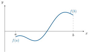
A continuous function with f(a) < 0 < f(b) must cross the axis: the dichotomy proof of  traps a crossing point between adjacent sequences.
A continuous function with f(a)<0<f(b)f(a) < 0 < f(b) must cross the axis: the dichotomy proof of Theorem 13.10 traps a crossing point between adjacent sequences.

উদাহরণ

Example 13.7 (A taxonomy of discontinuities)

Three ways to fail at a point, in increasing severity. Removable: f(x)=sin⁡xxf(x) = \frac{\sin x}{x} on R∗\R^* has limit 11 at 00; defining f(0)=1f(0) = 1 repairs it — the discontinuity was a hole, not a feature. Jump: ⌊x⌋\lfloor x \rfloor at an integer has distinct one-sided limits (n−1n - 1 and nn); no choice of value can reconcile them, but both half-limits exist. Essential: sin⁡1x\sin\frac1x at 00 has no one-sided limit at all (Exercise 13.1) — oscillation without settlement. Monotone functions can only produce the middle kind (their one-sided limits always exist, being suprema and infima), which is why their discontinuity sets are at most countable — one rational per jump. Derivatives, by Darboux’s theorem (Exercise 14.10), can only produce the last kind: a function with a jump discontinuity is never the derivative of anything.

Example 13.9 (Max and min of continuous functions)

If f,gf, g are continuous, so are max⁡(f,g)\max(f, g) and min⁡(f,g)\min(f, g): no case analysis needed, thanks to the identities

max⁡(f,g)=f+g+∣f−g∣2,min⁡(f,g)=f+g−∣f−g∣2,\max(f, g) = \frac{f + g + \abs{f - g}}{2}, \qquad \min(f, g) = \frac{f + g - \abs{f - g}}{2},

and the continuity of sums and of ∣ ⋅ ∣\abs{\,\cdot\,} (Proposition 13.8). In particular f+=max⁡(f,0)f^+ = \max(f, 0) and f−=max⁡(−f,0)f^- = \max(-f, 0) are continuous with f=f+−f−f = f^+ - f^-: the sign-splitting used for series (Chapter 17) and, at full scale, in the integration theory of the Year 3 volume, costs nothing in regularity.

Example 13.11 (One equation, the full protocol)

Solve ex=3−x\eu^x = 3 - x over R\R: existence, uniqueness, location. Set g(x)=ex+x−3g(x) = \eu^x + x - 3, continuous. Location and existence: g(0)=−2<0g(0) = -2 < 0 and g(1)=e−2>0g(1) = \eu - 2 > 0, so the intermediate value theorem plants a solution in (0, 1)\intoo{0}{1}. Uniqueness: gg is a sum of the strictly increasing ex\eu^x and x−3x - 3, hence strictly increasing on R\R; a strictly monotone function takes each value at most once, so the solution is unique on all of R\R (not just in the interval probed). The protocol — rearrange to g=0g = 0, sign change for existence, monotonicity for uniqueness — settles most “how many solutions” questions in three lines, and Chapter 14’s variation tables extend it to non-monotone gg by cutting R\R into monotone branches.

প্রসঙ্গসহ পড়ো →