High School Mathematics · Grades 10–12

21Limits and Continuity

This chapter extends the notion of limit from sequences to functions of a real variable, and introduces continuity. The central result is the intermediate value theorem, which turns qualitative information (“ $f$ is continuous and changes sign”) into the existence of solutions of equations.

21.1 Limits of functions

Throughout, $f$ is a function defined on an interval or a union of intervals $D \subseteq \R$ .

Definition 21.1 (Limit at infinity)

Let $f$ be defined on an interval $\intco{a}{+\infty}$ and $\ell \in \R$ . We say that $f$ tends to $\ell$ at $+\infty$ , written $\lim\limits_{x\to+\infty} f(x) = \ell$ , if every open interval containing $\ell$ contains all values $f(x)$ for $x$ large enough: for every $\varepsilon > 0$ there exists $A$ such that for all $x \geq A$ , $\abs{f(x) - \ell} \leq \varepsilon$ .

We say $f$ tends to $+\infty$ at $+\infty$ if for every $M \in \R$ there exists $A$ such that $f(x) \geq M$ for all $x \geq A$ . Limits at $-\infty$ and limits equal to $-\infty$ are defined analogously.

Definition 21.2 (Limit at a point)

Let $a \in \R$ and let $f$ be defined near $a$ (except possibly at $a$ ). We say that $f$ tends to $\ell \in \R$ at $a$ , written $\lim\limits_{x \to a} f(x) = \ell$ , if for every $\varepsilon > 0$ there exists $\delta > 0$ such that for all $x \in D$ with $\abs{x - a} \leq \delta$ , $\abs{f(x) - \ell} \leq \varepsilon$ .

We say $f$ tends to $+\infty$ at $a$ if for every $M$ there is $\delta > 0$ such that $f(x) \geq M$ whenever $x \in D$ and $\abs{x - a} \leq \delta$ . One-sided limits ( $x \to a^+$ , $x \to a^-$ ) restrict $x$ to $x > a$ or $x < a$ .

Example 21.3

$\lim\limits_{x\to+\infty} \frac{1}{x} = 0$ , $\lim\limits_{x\to 0^+} \frac{1}{x} = +\infty$ , $\lim\limits_{x\to 0^-} \frac{1}{x} = -\infty$ . The function $x \mapsto \frac1x$ has no (two-sided) limit at $0$ .

Definition 21.4 (Asymptotes)

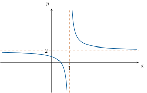
The line $y = \ell$ is a horizontal asymptote of the curve of $f$ at $+\infty$ (resp. $-\infty$ ) if $\lim_{x\to+\infty} f(x) = \ell$ (resp. at $-\infty$ ). The line $x = a$ is a vertical asymptote if $f$ has an infinite one-sided limit at $a$ .

The curve of f(x) = 2 + 1/x-1 with its horizontal asymptote y = 2 (at ±∈fty) and vertical asymptote x = 1. — The curve of $f(x) = 2 + \frac{1}{x-1}$ with its horizontal asymptote $y = 2$ (at $\pm\infty$ ) and vertical asymptote $x = 1$ .

Proposition 21.5 (Operations on limits)

The rules of Proposition 20.14 (sums, products, quotients) hold verbatim for limits of functions, at a point or at infinity, with the same four indeterminate forms $(+\infty)+(-\infty)$ , $0\times\infty$ , $\frac{\infty}{\infty}$ , $\frac{0}{0}$ .

Proof. The proofs are identical to the sequence case, replacing “for $n \geq N$ ” by “for $x \geq A$ ” or “for $\abs{x-a} \leq \delta$ ”. ∎

Theorem 21.6 (Limit of a composition)

Let $f, g$ be functions and $a, b, c$ be real numbers or $\pm\infty$ . If $\lim\limits_{x \to a} f(x) = b$ and $\lim\limits_{y \to b} g(y) = c$ , then

\lim_{x \to a} g\bigl(f(x)\bigr) = c .

The same statement holds with a sequence in place of $f$ : if $u_n \to b$ and $\lim_{y\to b} g(y) = c$ , then $g(u_n) \to c$ .

Proof. Take $b, c$ finite (the other cases are analogous). Let $\varepsilon > 0$ . There is $\delta > 0$ such that $\abs{y - b} \leq \delta$ implies $\abs{g(y) - c} \leq \varepsilon$ ; and there is $\delta' > 0$ such that $\abs{x - a} \leq \delta'$ implies $\abs{f(x) - b} \leq \delta$ . Chaining the two gives $\abs{g(f(x)) - c} \leq \varepsilon$ for $\abs{x - a} \leq \delta'$ . ∎

Theorem 21.7 (Comparison and squeeze)

Let $f, g, h$ be functions and $a \in \R \cup \{\pm\infty\}$ .

If $f \leq g$ near $a$ and $f(x) \to +\infty$ as $x \to a$ , then $g(x) \to +\infty$ .
If $f \leq g \leq h$ near $a$ and $f, h$ tend to the same finite limit $\ell$ at $a$ , then $g(x) \to \ell$ as $x \to a$ .

Proof. Same argument as for sequences (Theorem 20.16). ∎

Method 21.8 (Computing limits in practice)

Polynomials and rational functions at $\pm\infty$ : factor out the highest power of $x$ ; the limit is that of the ratio of leading terms.
$\frac{0}{0}$ at a point $a$ : factor $(x-a)$ out of numerator and denominator, or recognize a derivative $\lim_{x\to a}\frac{f(x)-f(a)}{x-a} = f'(a)$ (Chapter 22).
Square roots: multiply by the conjugate expression.
Oscillating factors ( $\cos$ , $\sin$ ): use the squeeze theorem.

21.2 Continuity

Definition 21.9 (Continuity)

Let $f$ be defined on an interval $I$ and $a \in I$ . The function $f$ is continuous at $a$ if $\lim\limits_{x \to a} f(x) = f(a)$ . It is continuous on $I$ if it is continuous at every point of $I$ .

Intuitively, the graph of a continuous function on an interval can be drawn without lifting the pen.

Proposition 21.10 (Continuity of usual functions)

Polynomials, rational functions, $x \mapsto \sqrt{x}$ , $x \mapsto \abs{x}$ , $\cos$ , $\sin$ , $\exp$ and $\ln$ are continuous on every interval contained in their domain. Sums, products, quotients (where defined) and compositions of continuous functions are continuous.

Partial proof. Stability under sums, products, quotients and composition follows from the corresponding theorems on limits. Continuity of $x \mapsto x$ and of constant functions is immediate from the definition, hence polynomials and rational functions are continuous. Continuity of the remaining usual functions is proved in the chapters where they are constructed, or admitted. ∎

Example 21.11

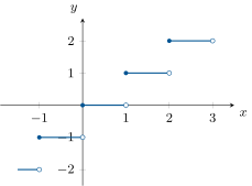
The floor function $x \mapsto \floor{x}$ (the greatest integer $\leq x$ ) is not continuous at any integer $n$ : its left limit there is $n - 1$ while $\floor{n} = n$ .

The floor function jumps at each integer: the value (filled dot) differs from the left limit (open dot).

Proposition 21.12 (Sequences and continuity)

If $u_n \to \ell$ and $f$ is continuous at $\ell$ , then $f(u_n) \to f(\ell)$ . In particular, if a sequence defined by $u_{n+1} = f(u_n)$ converges to $\ell$ and $f$ is continuous at $\ell$ , then $f(\ell) = \ell$ .

Proof. The first claim is Theorem 21.6 applied with the sequence $(u_n)$ . For the second, pass to the limit on both sides of $u_{n+1} = f(u_n)$ : the left side tends to $\ell$ , the right side to $f(\ell)$ , and limits are unique. ∎

21.3 The intermediate value theorem

Theorem 21.13 (Intermediate value theorem)

Let $f$ be continuous on $\intcc{a}{b}$ and let $k$ be any number between $f(a)$ and $f(b)$ . Then there exists $c \in \intcc{a}{b}$ such that $f(c) = k$ .

The intermediate value theorem: a continuous curve joining (a, f(a)) to (b, f(b)) must cross every horizontal line y = k lying between f(a) and f(b). — The intermediate value theorem: a continuous curve joining $(a, f(a))$ to $(b, f(b))$ must cross every horizontal line $y = k$ lying between $f(a)$ and $f(b)$ .

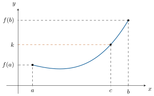
Proof. Replacing $f$ by $f - k$ (and by $k - f$ if needed), we may assume $f(a) \leq 0 \leq f(b)$ and look for a zero of $f$ . We construct two sequences by dichotomy: set $a_0 = a$ , $b_0 = b$ ; given $a_n \leq b_n$ with $f(a_n) \leq 0 \leq f(b_n)$ , let $m = \frac{a_n + b_n}{2}$ and define

(a_{n+1}, b_{n+1}) = \begin{cases} (a_n, m) & \text{if } f(m) \geq 0,\\ (m, b_n) & \text{if } f(m) < 0. \end{cases}

In both cases $f(a_{n+1}) \leq 0 \leq f(b_{n+1})$ , the sequence $(a_n)$ is increasing, $(b_n)$ is decreasing, and $b_n - a_n = \frac{b-a}{2^n} \to 0$ : the sequences are adjacent (see Exercise 20.10) and converge to a common limit $c \in \intcc{a}{b}$ . By continuity, $f(a_n) \to f(c)$ and $f(b_n) \to f(c)$ ; passing to the limit in $f(a_n) \leq 0$ and $f(b_n) \geq 0$ gives $f(c) \leq 0 \leq f(c)$ , so $f(c) = 0$ . ∎

Remark 21.14

The dichotomy proof is an algorithm: it yields arbitrarily precise approximations of a solution, halving the error at each step. This is how a computer can solve $f(x) = 0$ knowing only how to evaluate $f$ .

Theorem 21.15 (Bijection theorem)

Let $f$ be continuous and strictly monotonic on an interval $I$ . Then for every $k$ strictly between the limits of $f$ at the endpoints of $I$ , the equation $f(x) = k$ has a unique solution in $I$ .

Proof. Existence: choose $a, b \in I$ with $k$ between $f(a)$ and $f(b)$ (possible since the values of $f$ approach its endpoint limits), and apply the intermediate value theorem on $\intcc{a}{b}$ . Uniqueness: if $x < y$ , strict monotonicity gives $f(x) \neq f(y)$ , so two distinct points cannot both be solutions. ∎

Method 21.16 (Solving $f(x) = k$ with the bijection theorem)

To prove that $f(x) = k$ has exactly one solution in an interval:

establish a variation table of $f$ (sign of $f'$ , see Chapter 22);
on each interval where $f$ is continuous and strictly monotonic, compare $k$ with the endpoint values or limits;
apply the bijection theorem on each such interval and count the solutions.

A calculator or dichotomy then localizes each solution as finely as desired.

Example 21.17

The equation $x^3 + x = 1$ has a unique real solution. Indeed $f(x) = x^3 + x$ is continuous and strictly increasing on $\R$ (as a sum of strictly increasing functions), $\lim_{-\infty} f = -\infty$ and $\lim_{+\infty} f = +\infty$ , so the bijection theorem applies with $k = 1$ . Since $f(0.6) = 0.816 < 1$ and $f(0.7) = 1.043 > 1$ , the solution lies in $\intoo{0.6}{0.7}$ .

21.4 Exercises

Exercise 21.1 ★

Compute the following limits:

\lim_{x\to+\infty} \frac{2x^3 - x + 1}{5x^3 + x^2}, \qquad \lim_{x\to-\infty} \bigl(x^2 + 3x - 1\bigr), \qquad \lim_{x\to 2^+} \frac{x+1}{x-2}, \qquad \lim_{x\to+\infty} \frac{\cos x}{x}.

Solution

Solution of Exercise 21.1.

Dividing by $x^3$ : $\dfrac{2x^3 - x + 1}{5x^3 + x^2} = \dfrac{2 - 1/x^2 + 1/x^3}{5 + 1/x} \to \dfrac{2}{5}$ .

$x^2 + 3x - 1 = x^2(1 + 3/x - 1/x^2) \to +\infty$ as $x \to -\infty$ , since $x^2 \to +\infty$ and the bracket tends to $1$ .

As $x \to 2^+$ , the numerator tends to $3 > 0$ and the denominator to $0^+$ , so $\dfrac{x+1}{x-2} \to +\infty$ .

For $x > 0$ , $-\dfrac1x \leq \dfrac{\cos x}{x} \leq \dfrac1x$ , so the limit is $0$ by the squeeze theorem.

Exercise 21.2 ★

Let $f(x) = \dfrac{2x^2 - 3x + 1}{x - 1}$ , defined for $x \neq 1$ .

Show that $f(x) = 2x - 1$ for all $x \neq 1$ .
Deduce $\lim\limits_{x \to 1} f(x)$ . Can $f$ be extended to a function continuous at $1$ ?

Solution

Solution of Exercise 21.2.

1. $2x^2 - 3x + 1 = (x-1)(2x-1)$ (the root $x=1$ is apparent from $2 - 3 + 1 = 0$ ). For $x \neq 1$ , cancel $x - 1$ : $f(x) = 2x - 1$ .

2. Hence $\lim_{x\to1} f(x) = 1$ . Setting $f(1) = 1$ extends $f$ to the polynomial function $x \mapsto 2x-1$ on $\R$ , which is continuous at $1$ .

Exercise 21.3 ★

Determine the asymptotes of the curve of $f(x) = \dfrac{3x - 1}{x + 2}$ and sketch the curve.

Solution

Solution of Exercise 21.3.

Write $f(x) = \dfrac{3x - 1}{x + 2} = \dfrac{3(x+2) - 7}{x+2} = 3 - \dfrac{7}{x+2}$ . As $x \to \pm\infty$ , $f(x) \to 3$ : the line $y = 3$ is a horizontal asymptote at both infinities. As $x \to (-2)^\pm$ , $f(x) \to \mp\infty$ : the line $x = -2$ is a vertical asymptote. The curve is a hyperbola, below $y=3$ for $x > -2$ and above it for $x < -2$ .

Exercise 21.4 ★★

Compute

\lim_{x\to+\infty} \bigl(\sqrt{x^2 + x} - x\bigr) \qquad\text{and}\qquad \lim_{x\to 0} \frac{\sqrt{1+x} - 1}{x}.

Solution

Solution of Exercise 21.4.

Multiply by the conjugate:

\sqrt{x^2 + x} - x = \frac{x^2 + x - x^2}{\sqrt{x^2+x} + x} = \frac{x}{x\left(\sqrt{1 + 1/x} + 1\right)} = \frac{1}{\sqrt{1 + 1/x} + 1} \xrightarrow[x\to+\infty]{} \frac{1}{2}.

Similarly,

\frac{\sqrt{1+x} - 1}{x} = \frac{(1+x) - 1}{x\left(\sqrt{1+x} + 1\right)} = \frac{1}{\sqrt{1+x} + 1} \xrightarrow[x\to0]{} \frac{1}{2}.

Exercise 21.5 ★★

Let $f(x) = x + \sin x$ .

Show that $f(x) \to +\infty$ as $x \to +\infty$ , although $f$ is not monotonic on any interval $\intco{A}{+\infty}$ .
Show that $g(x) = \dfrac{x + \sin x}{x - \sin x}$ tends to $1$ at $+\infty$ .

Solution

Solution of Exercise 21.5.

1. Since $\sin x \geq -1$ , $f(x) \geq x - 1 \to +\infty$ , and we conclude by comparison. Yet $f'(x) = 1 + \cos x$ vanishes at every odd multiple of $\pi$ , and on every interval $\intco{A}{+\infty}$ the function alternates between intervals of strict increase; it is increasing but not strictly, and more importantly its growth is not needed: comparison suffices.

2. For $x > 1$ , divide by $x$ :

g(x) = \frac{1 + \frac{\sin x}{x}}{1 - \frac{\sin x}{x}},

and $\frac{\sin x}{x} \to 0$ by the squeeze theorem ( $\abs{\sin x} \leq 1$ ). Hence $g(x) \to \frac{1+0}{1-0} = 1$ .

Exercise 21.6 ★★

Show that the equation $x^3 - 3x + 1 = 0$ has exactly three real solutions, and give for each an interval of length $1$ containing it. (Hint: study the variations of $f(x) = x^3 - 3x + 1$ ; its derivative is $3x^2 - 3$ .)

Solution

Solution of Exercise 21.6.

$f(x) = x^3 - 3x + 1$ is continuous, with $f'(x) = 3x^2 - 3 = 3(x-1)(x+1)$ : $f$ increases on $\intoc{-\infty}{-1}$ , decreases on $\intcc{-1}{1}$ , increases on $\intco{1}{+\infty}$ , with local maximum $f(-1) = 3 > 0$ and local minimum $f(1) = -1 < 0$ , $\lim_{-\infty} f = -\infty$ , $\lim_{+\infty} f = +\infty$ .

On each of the three monotonicity intervals, $f$ is continuous, strictly monotonic, and $0$ lies strictly between the endpoint values/limits, so the bijection theorem gives exactly one zero per interval: three zeros in total. Sign checks: $f(-2) = -1 < 0 < f(-1) = 3$ , so one zero in $\intoo{-2}{-1}$ ; $f(0) = 1 > 0 > f(1) = -1$ , one zero in $\intoo{0}{1}$ ; $f(1) = -1 < 0 < f(2) = 3$ , one zero in $\intoo{1}{2}$ .

Exercise 21.7 ★★

Let $f \colon \intcc{0}{1} \to \intcc{0}{1}$ be continuous. Show that $f$ has a fixed point: there exists $c \in \intcc{0}{1}$ with $f(c) = c$ . (Hint: apply the intermediate value theorem to $g(x) = f(x) - x$ .)

Solution

Solution of Exercise 21.7.

Let $g(x) = f(x) - x$ , continuous on $\intcc{0}{1}$ . Since $f(0) \in \intcc{0}{1}$ , $g(0) = f(0) \geq 0$ ; since $f(1) \in \intcc{0}{1}$ , $g(1) = f(1) - 1 \leq 0$ . By the intermediate value theorem, $g$ vanishes at some $c \in \intcc{0}{1}$ , i.e. $f(c) = c$ .

Exercise 21.8 ★★★

A hiker climbs a mountain trail, starting at 8:00 and arriving at 20:00. The next day she descends the same trail, again starting at 8:00 and arriving at 20:00. Show that there is a time of day at which she is at exactly the same point of the trail on both days. (Hint: introduce the difference of the two position functions.)

Solution

Solution of Exercise 21.8.

Let $u(t)$ and $d(t)$ be the positions (measured as distance from the bottom of the trail) at time $t \in \intcc{8}{20}$ on the way up and on the way down. Both are continuous, $u(8) = 0$ , $u(20) = L$ (the length of the trail), $d(8) = L$ , $d(20) = 0$ . The function $g = u - d$ is continuous with $g(8) = -L \leq 0$ and $g(20) = L \geq 0$ , so $g(c) = 0$ for some time $c$ by the intermediate value theorem: at time $c$ , both days’ positions coincide.

Exercise 21.9 ★★★

Let $f(x) = x^5 + x^3 + x - 1$ .

Show that $f$ has a unique real zero $\alpha$ , and that $\alpha \in \intoo{0}{1}$ .
Describe a dichotomy procedure computing $\alpha$ to within $10^{-6}$ , and give the number of iterations required starting from $\intcc{0}{1}$ .

Solution

Solution of Exercise 21.9.

1. $f'(x) = 5x^4 + 3x^2 + 1 > 0$ , so $f$ is strictly increasing on $\R$ ; with $\lim_{\pm\infty} f = \pm\infty$ and continuity, the bijection theorem gives a unique real zero $\alpha$ . Since $f(0) = -1 < 0$ and $f(1) = 2 > 0$ , $\alpha \in \intoo{0}{1}$ .

2. Maintain an interval $\intcc{a_n}{b_n}$ with $f(a_n) < 0 < f(b_n)$ , starting from $\intcc{0}{1}$ ; at each step evaluate $f$ at the midpoint $m$ and keep the half-interval on which the sign change persists. After $n$ steps the interval has length $2^{-n}$ , so the midpoint approximates $\alpha$ to within $2^{-(n+1)}$ . We need $2^{-(n+1)} \leq 10^{-6}$ , i.e. $n + 1 \geq \frac{6}{\log_{10} 2} \approx 19.93$ : $n = 20$ iterations suffice.

21.5 Problem: You cannot cross a river without getting wet

Problem 21.1

Weekend problem — the intermediate value theorem forces fixed points, equal-temperature antipodes and steady tables: three impossible-sounding theorems from one idea

Crumple a map of France and drop it anywhere on French soil: some point of the map lies exactly above the place it represents. At every instant, two diametrically opposite points of the equator have exactly the same temperature. And a wobbly square table on bumpy ground can always be steadied by rotating it. Three party tricks, one theorem: a continuous quantity cannot pass from negative to positive without vanishing (Theorem 21.13). This problem trains limits, then builds all three wonders — and knows exactly what the theorem does not promise.

Part I — Limit fluency.

Compute $\lim_{x \to +\infty} \dfrac{3x^2 - x}{x^2 + 5}$ , $\lim_{x \to +\infty} \dfrac{2x + 1}{x^2 + 1}$ , and $\lim_{x \to +\infty} (x^3 - x^2)$ (Method 21.8).
Give the asymptotes of $f(x) = \dfrac{3x - 1}{x + 2}$ (Definition 21.4), computing the relevant limits.
Compute $\lim_{x \to 3} \dfrac{x^2 - 9}{x - 3}$ (factor) and $\lim_{x \to 0} \dfrac{\sqrt{x + 1} - 1}{x}$ (conjugate).
By the squeeze theorem (Theorem 21.7): compute $\lim_{x \to 0} x \sin\frac1x$ and $\lim_{x \to +\infty} \frac{\sin x}{x}$ .
By composition and dominant terms: $\lim_{x \to +\infty} \dfrac{\sqrt{4x^2 + x}}{x}$ .

Part II — Roots, certified.

Show that the equation $x^3 + x = 5$ has at least one solution in $\intcc{1}{2}$ .
Show the solution is unique on $\R$ (Theorem 21.15).
Prove the classic: every polynomial of odd degree has at least one real root. (Write out the argument for $p(x) = x^3 + a x^2 + b x + c$ : compute the two infinite limits by dominant term, then apply the IVT on a large interval.)
Locating the root of question 6 by dichotomy: how many halvings of $\intcc{1}{2}$ guarantee an error below $10^{-6}$ (Exercise 21.9)? Compare with the digit-doubling of Newton’s method (Problem 12.1): roughly how many steps would it need?
The counterexample that guards the theorem: $g(x) = \frac1x$ satisfies $g(-1) = -1 < 0$ and $g(1) = 1 > 0$ , yet never vanishes. Which hypothesis of the IVT fails — and what does the example teach about checking hypotheses?

Part III — Three impossible-sounding theorems.

The fixed-point theorem of the segment: if $f : \intcc{0}{1} \to \intcc{0}{1}$ is continuous, prove that some $c$ satisfies $f(c) = c$ . (Study $g(x) = f(x) - x$ at the two ends.)
Translate question 11 into the crumpled map: what plays the role of $f$ , why does it land in $\intcc{0}{1}$ (figuratively: within France), and what is the point lying exactly above its own location? (One dimension is admitted silently — the honest two-dimensional statement is Brouwer’s theorem, university volumes.)
The equator: let $T$ be a continuous temperature on a circle, seen as a $2\pi$ -periodic function with $T(0) = T(2\pi)$ . Set $g(t) = T(t) - T(t + \pi)$ . Compute $g(0) + g(\pi)$ , deduce that $g$ vanishes somewhere on $\intcc{0}{\pi}$ , and state the theorem about antipodal points.
The wobbly table: a perfectly rigid square table stands on continuous (no steps!) bumpy ground; three legs always touch, one hovers by a height $h(\theta)$ that depends continuously on the table’s rotation angle $\theta$ . Explain why rotating by a quarter turn forces the hovering gap to change sign — and conclude that some angle $\theta^*$ steadies all four legs. (This argument was published as a genuine theorem in 2005; café owners knew the trick first.)
The hiker of Exercise 21.8 used the same scheme. State the template shared by questions 11, 13, 14 and the hiker — build which function, check what at the ends, invoke what — in three lines.
What the IVT does not give: existence came free, but which two questions does it leave open, and which tools of this problem answer them (questions 7 and 9)?

Part IV — Portraits with asymptotes.

Rewrite $f(x) = \dfrac{3x - 1}{x + 2}$ as $3 - \dfrac{7}{x + 2}$ and use it to describe the curve completely: asymptotes, variations on each side, sketch. (A shifted hyperbola — the average-cost curve of Problem 4.1 was one too.)
The function $f(x) = \dfrac{x^2 - 1}{x - 1}$ is undefined at $1$ . Which value assigned to $f(1)$ makes it continuous there — and why do analysts call such a point a removable discontinuity?
The floor function $x \mapsto \lfloor x \rfloor$ (greatest integer $\leq x$ ): where is it continuous, where does it jump, and why does the IVT’s conclusion fail for it (find $a < b$ with $\lfloor a \rfloor < \frac12 < \lfloor b \rfloor$ yet no solution of $\lfloor x \rfloor = \frac12$ )?
Finale — continuity’s two faces: the local promise (value $=$ limit: no teleporting) and the global power (IVT: every intermediate value visited). File the four wonders of Part III under the right face, and give the river-crossing slogan its precise mathematical name.

Solution

Solution of Problem 21.1.

1. Dominant terms: $\frac{3x^2}{x^2} \to 3$ ; $\frac{2x}{x^2} = \frac2x \to 0$ ; $x^3 - x^2 = x^3\left(1 - \frac1x\right) \to +\infty$ .

2. $\lim_{x \to \pm\infty} f = 3$ : horizontal asymptote $y = 3$ ; $\lim_{x \to (-2)^\pm} f = \mp\infty$ : vertical asymptote $x = -2$ .

3. $\frac{(x-3)(x+3)}{x - 3} = x + 3 \to 6$ . And $\frac{\sqrt{x+1} - 1}{x} = \frac{x}{x(\sqrt{x+1} + 1)} = \frac{1}{\sqrt{x+1} + 1} \to \frac12$ .

4. $\abs{x \sin\frac1x} \leq \abs x \to 0$ , so the limit is $0$ . And $\abs{\frac{\sin x}{x}} \leq \frac1x \to 0$ : limit $0$ .

5. $\frac{\sqrt{4x^2 + x}}{x} = \sqrt{4 + \frac1x} \to \sqrt4 = 2$ (continuity of the square root, composition).

6. $f(x) = x^3 + x$ is continuous with $f(1) = 2 < 5 < 10 = f(2)$ : by the IVT, $f(c) = 5$ for some $c \in \intoo{1}{2}$ .

7. $f'(x) = 3x^2 + 1 > 0$ : strictly increasing on $\R$ , continuous, with limits $\mp\infty$ : by the bijection theorem, every value — in particular $5$ — is attained exactly once.

8. $p(x) = x^3\left(1 + \frac ax + \frac{b}{x^2} + \frac{c}{x^3}\right)$ : as $x \to +\infty$ , $p \to +\infty$ ; as $x \to -\infty$ , $p \to -\infty$ . So on some huge interval $\intcc{-M}{M}$ , $p(-M) < 0 < p(M)$ : the IVT delivers a root. The same dominant-term argument works verbatim for any odd degree — odd powers keep opposite signs at the two infinities.

9. Halving $n$ times leaves an interval of length $2^{-n}$ ; $2^{-20} \approx 9.5 \times 10^{-7} < 10^{-6}$ : twenty steps. Newton doubles correct digits each step: from one correct digit, about $3$ – $4$ steps reach six — the tortoise and the greyhound of root-finding.

10. $g$ is not continuous on $\intcc{-1}{1}$ : it explodes at $0$ , which the interval contains. The IVT’s conclusion evaporates with its hypothesis — always check continuity on the whole interval, not just at the endpoints.

11. $g(x) = f(x) - x$ is continuous; $g(0) = f(0) \geq 0$ (values lie in $\intcc{0}{1}$ ) and $g(1) = f(1) - 1 \leq 0$ . By the IVT, $g(c) = 0$ for some $c$ : $f(c) = c$ .

12. Idealizing the country as the segment $\intcc{0}{1}$ : $f$ sends each place to the place shown directly beneath it on the crumpled map; crumpling keeps the map over the country, so $f$ lands in $\intcc{0}{1}$ , and it is continuous (paper does not tear). The fixed point $c$ is the spot lying precisely above its own image — Brouwer’s theorem handles the honest two-dimensional map.

13. $g(0) + g(\pi) = \left(T(0) - T(\pi)\right) + \left(T(\pi) - T(2\pi)\right) = T(0) - T(2\pi) = 0$ . So $g(0)$ and $g(\pi)$ are opposite (or both zero): either way $g$ , continuous, vanishes at some $t^* \in \intcc{0}{\pi}$ : $T(t^*) = T(t^* + \pi)$ — somewhere on the equator, two antipodal points agree on the temperature, at every single moment.

14. Rotating the table by a quarter turn exchanges the roles of the two diagonals: the pair of legs that pressed the ground and the pair that (one of them) hovered swap situations, so the hovering height — counted with its sign as “gap of the distinguished diagonal” — takes opposite signs at $\theta$ and $\theta + \frac\pi2$ . Continuous ground makes $h$ continuous, and the IVT hands over an angle $\theta^*$ with $h(\theta^*) = 0$ : four legs down. (No such luck with a rectangular table or stepped ground.)

15. Template: build the difference of the two quantities you want to coincide ( $f(x) - x$ ; $T(t) - T(t + \pi)$ ; up-position minus down-position for the hiker; the signed gap for the table); check it takes values of both signs (often via a symmetry of the ends); invoke the IVT on a continuous function. Coincidence forced.

16. Open questions: how many solutions (answered by strict monotonicity and the bijection theorem, question 7) and where they are (answered by dichotomy or Newton, question 9). The IVT is a pure existence oracle.

17. $3 - \frac{7}{x + 2}$ : vertical asymptote $x = -2$ , horizontal $y = 3$ ; on each side of $-2$ the function is increasing ( $-\frac{7}{x+2}$ increases where defined); the curve is the reference hyperbola $-\frac7x$ shifted left $2$ and up $3$ — two branches hugging the asymptote cross.

18. For $x \neq 1$ : $f(x) = x + 1$ , so $\lim_{x \to 1} f = 2$ : setting $f(1) = 2$ restores continuity. The discontinuity was a puncture, not a jump — fill the single missing point and the curve heals: removable.

19. Continuous on every interval between consecutive integers; at each integer $n$ it jumps from $n - 1$ to $n$ . With $a = 0.9$ , $b = 1.1$ : $\lfloor a \rfloor = 0 < \frac12 < 1 = \lfloor b \rfloor$ , yet $\lfloor x \rfloor = \frac12$ has no solution — the jump teleports over $\frac12$ , which is precisely what the IVT forbids continuous functions to do.

20. Local face: value $=$ limit at each point — the removable puncture (question 18) violated it curably, the floor’s jumps (question 19) incurably. Global face: on an interval, all intermediate values are visited — the root certificates (6–8), the fixed point, the equator, the table and the hiker all live here. The slogan’s official name: the intermediate value theorem.