University Mathematics — Year 1 · Bachelor Year 1

14Differentiation

Derivatives were computed throughout the High School volume; what was missing is the chain of theorems that turns computation into information about functions: Rolle’s theorem, the mean value theorem, and their consequences — monotonicity criteria, Lipschitz bounds, convexity. Everything in this chapter concerns functions defined on an interval $I$ .

14.1 The derivative

Definition 14.1

$f \colon I \to \R$ is differentiable at $x_0 \in I$ when the difference quotient $\frac{f(x) - f(x_0)}{x - x_0}$ has a (finite) limit as $x \to x_0$ ; the limit is written $f'(x_0)$ . Equivalently:

f(x_0 + h) = f(x_0) + f'(x_0)\,h + h\,\varepsilon(h), \qquad \varepsilon(h) \xrightarrow[h \to 0]{} 0 ,

the graph then admitting the tangent line $y = f(x_0) + f'(x_0)(x - x_0)$ . Differentiability at $x_0$ implies continuity at $x_0$ (read the display). $f$ is differentiable on $I$ when it is at every point; $f$ is of class $C^1$ when moreover $f'$ is continuous, and of class $C^k$ when $f$ can be differentiated $k$ times with $f^{(k)}$ continuous.

Example 14.2

The converse of “differentiable $\Rightarrow$ continuous” fails: $\abs{\,\cdot\,}$ at $0$ . More surprisingly, differentiable does not imply $C^1$ : the function $f(x) = x^2 \sin\frac 1x$ ( $f(0) = 0$ ) is differentiable everywhere, with $f'(0) = 0$ , but $f'(x) = 2x \sin\frac1x - \cos\frac 1x$ has no limit at $0$ (Exercise 14.2).

Example 14.3 (Differentiable at exactly one point)

Let $f(x) = x^2$ for $x \in \Q$ and $f(x) = 0$ for $x \notin \Q$ . At $0$ : $\bigl|\frac{f(h) - 0}{h}\bigr| \leq \abs h \to 0$ , so $f$ is differentiable at $0$ with $f'(0) = 0$ . At any $x_0 \neq 0$ , $f$ is not even continuous: rational and irrational sequences converging to $x_0$ send $f$ to $x_0^2 \neq 0$ and to $0$ respectively (density, Theorem 10.14). So differentiability is a genuinely pointwise notion: it can hold at one point of $\R$ and nowhere else. The moral for practice: statements like the monotonicity criterion or Rolle require the derivative on an interval — possessing $f'(x_0)$ at isolated points, however many, supports no global conclusion whatsoever.

Theorem 14.4 (Operations)

If $f, g$ are differentiable at $x_0$ (and where the formulas make sense):

(f + g)' = f' + g', \qquad (fg)' = f'g + fg', \qquad \Bigl(\frac fg\Bigr)' = \frac{f'g - fg'}{g^2},

and if $g$ is differentiable at $f(x_0)$ : $\;(g \circ f)'(x_0) = g'\bigl(f(x_0)\bigr)\, f'(x_0)$ (chain rule).

Proof. Sum: immediate. Product: write

f(x)g(x) - f(x_0)g(x_0) = \bigl(f(x) - f(x_0)\bigr) g(x) + f(x_0)\bigl(g(x) - g(x_0)\bigr),

divide by $x - x_0$ and let $x \to x_0$ ( $g$ is continuous at $x_0$ ). Quotient: treat $\frac 1g$ via $\frac{1/g(x) - 1/g(x_0)}{x - x_0} = \frac{-1}{g(x)g(x_0)}\cdot\frac{g(x) - g(x_0)}{x - x_0}$ , then apply the product rule. Chain rule: with $y_0 = f(x_0)$ , define $\theta(y) = \frac{g(y) - g(y_0)}{y - y_0}$ for $y \neq y_0$ and $\theta(y_0) = g'(y_0)$ : $\theta$ is continuous at $y_0$ , and for $x \neq x_0$ ,

\frac{g(f(x)) - g(f(x_0))}{x - x_0} = \theta\bigl(f(x)\bigr)\cdot \frac{f(x) - f(x_0)}{x - x_0} \longrightarrow g'(y_0)\, f'(x_0),

the first factor by composition of limits (this device handles the case $f(x) = f(x_0)$ cleanly, where the naive “multiply and divide by $f(x) - f(x_0)$ ” breaks). ∎

Theorem 14.5 (Derivative of an inverse function)

Let $f$ be continuous and strictly monotonic on $I$ , differentiable at $x_0$ with $f'(x_0) \neq 0$ . Then $f^{-1}$ (Theorem 13.16) is differentiable at $y_0 = f(x_0)$ , with

(f^{-1})'(y_0) = \frac{1}{f'(x_0)} = \frac{1}{f'\bigl(f^{-1}(y_0)\bigr)} .

If $f'(x_0) = 0$ , the inverse has a vertical tangent at $y_0$ .

Proof. For $y \to y_0$ , set $x = f^{-1}(y)$ : continuity of $f^{-1}$ gives $x \to x_0$ , and

\frac{f^{-1}(y) - f^{-1}(y_0)}{y - y_0} = \frac{x - x_0}{f(x) - f(x_0)} = \frac{1}{\dfrac{f(x) - f(x_0)}{x - x_0}} \longrightarrow \frac{1}{f'(x_0)} .

Vertical-tangent claim: if $f'(x_0) = 0$ , the displayed quotient is the reciprocal of a quantity that tends to $0$ while keeping one constant sign (for $f$ strictly increasing, $\frac{f(x) - f(x_0)}{x - x_0} > 0$ for all $x \neq x_0$ ): the difference quotient of $f^{-1}$ therefore tends to $+\infty$ (to $-\infty$ for $f$ decreasing). The inverse remains continuous but is not differentiable at $y_0$ — its graph, the reflection of $f$ ’s across the diagonal, stands vertical exactly where $f$ ’s ran horizontal, as $x^{1/3}$ at $0$ illustrates against $x^3$ . ∎

Example 14.6 (Inverse derivatives, twice)

The theorem recomputes the classical derivatives with no limit work. For $\ln = \exp^{-1}$ : at $y = \eu^x$ ,

(\ln)'(y) = \frac{1}{\exp'(x)} = \frac{1}{\eu^{x}} = \frac1y ,

valid for every $y > 0$ since $\exp' = \exp$ never vanishes. For $\arctan = \tan^{-1}$ : at $y = \tan x$ ,

(\arctan)'(y) = \frac{1}{1 + \tan^2 x} = \frac{1}{1 + y^2} ,

using $\tan' = 1 + \tan^2 > 0$ . The closing insight: the formula converts knowledge about a function into knowledge about its inverse at the price of one substitution — and the substitution ( $x = \ln y$ , $x = \arctan y$ ) is exactly the statement that the two variables live on opposite sides of the bijection.

14.2 Rolle and the mean value theorem

Proposition 14.7 (Interior extremum)

If $f$ is differentiable at an interior point $x_0$ of $I$ and has a local extremum there, then $f'(x_0) = 0$ .

Proof. Say a local maximum: there is $r > 0$ with $f(x) \leq f(x_0)$ for $\abs{x - x_0} \leq r$ , and interiority guarantees both sides of $x_0$ are available within $I$ . For $0 < h \leq r$ the quotient $\frac{f(x_0 + h) - f(x_0)}{h}$ has numerator $\leq 0$ and denominator $> 0$ : it is $\leq 0$ , and its limit $f'(x_0)$ inherits $\leq 0$ (wide inequalities pass to limits, Theorem 11.7); for $-r \leq h < 0$ the quotient is $\geq 0$ , giving $f'(x_0) \geq 0$ . Hence $f'(x_0) = 0$ . (At an endpoint, only one sign is available: the conclusion fails there — think of $x$ on $\intcc{0}{1}$ , maximal at $1$ with derivative $1$ .) ∎

Theorem 14.8 (Rolle)

Let $f$ be continuous on $\intcc{a}{b}$ , differentiable on $\intoo{a}{b}$ , with $f(a) = f(b)$ . Then $f'(c) = 0$ for some $c \in \intoo{a}{b}$ .

Proof. By the extreme value theorem (Theorem 13.13), $f$ attains its maximum and minimum on $\intcc{a}{b}$ . If both are attained at endpoints, then (since $f(a) = f(b)$ ) max $=$ min and $f$ is constant: any interior $c$ works. Otherwise an extremum is attained at an interior point $c$ , and Proposition 14.7 gives $f'(c) = 0$ . ∎

Theorem 14.9 (Mean value theorem)

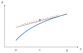
Let $f$ be continuous on $\intcc{a}{b}$ , differentiable on $\intoo{a}{b}$ . There exists $c \in \intoo{a}{b}$ with

f(b) - f(a) = f'(c)\,(b - a) .

Mean value inequality: if moreover $m \leq f' \leq M$ on $\intoo{a}{b}$ , then $m(b-a) \leq f(b) - f(a) \leq M(b-a)$ ; in particular $\abs{f'} \leq K$ implies that $f$ is $K$ -Lipschitz.

Proof. Apply Rolle to $g(x) = f(x) - \frac{f(b) - f(a)}{b - a}(x - a)$ : $g$ is continuous on $\intcc{a}{b}$ , differentiable inside, and $g(a) = f(a) = g(b)$ . At the point $c$ where $g'(c) = 0$ : $f'(c) = \frac{f(b)-f(a)}{b-a}$ . The inequality follows by bounding $f'(c)$ ; the Lipschitz statement applies it to every pair of points. ∎

The mean value theorem: some tangent (dashed) is parallel to the chord (gray). Its abscissa c is where Rolle’s theorem, applied to the function minus its chord, finds a critical point. — The mean value theorem: some tangent (dashed) is parallel to the chord (gray). Its abscissa $c$ is where Rolle’s theorem, applied to the function minus its chord, finds a critical point.

Example 14.10 (Newton’s method is Heron’s)

Newton’s method for solving $f(x) = 0$ replaces the curve by its tangent at the current guess $x_n$ and takes the tangent’s root as the next guess:

0 = f(x_n) + f'(x_n)(x_{n+1} - x_n) \quad\Longrightarrow\quad x_{n+1} = x_n - \frac{f(x_n)}{f'(x_n)} .

Run it on $f(x) = x^2 - 2$ :

x_{n+1} = x_n - \frac{x_n^2 - 2}{2x_n} = \frac{x_n}{2} + \frac{1}{x_n} = \frac12\Bigl(x_n + \frac{2}{x_n}\Bigr) :

exactly Heron’s iteration (Example 11.24), two millennia early. The quadratic speed observed there is now explained by the tangent picture: near a simple root, curve and tangent differ by a second-order error, so each step roughly squares the error — the general statement follows from the Taylor bounds of Chapter 16. The closing insight: where dichotomy (Example 13.12) uses only continuity and gains one bit per step, Newton spends a derivative to double the number of correct digits per step.

Example 14.11 (The mean value theorem as an estimator)

How large is $\sqrt{101}$ ? Apply the theorem to $f(t) = \sqrt t$ on $\intcc{100}{101}$ : for some $c \in \intoo{100}{101}$ ,

\sqrt{101} - 10 = \frac{1}{2\sqrt c}, \qquad\text{so}\qquad \frac{1}{2\sqrt{101}} < \sqrt{101} - 10 < \frac{1}{20} = 0.05 ,

and since $\sqrt{101} < 10.05$ , the left bound exceeds $\frac{1}{20.1} > 0.0497$ : thus $10.0497 < \sqrt{101} < 10.05$ (true value $10.049875\dots$ ) — three correct decimals from one derivative evaluation. Likewise $\abs{\sin a - \sin b} \leq \abs{a - b}$ (bound $\abs{\cos}\leq 1$ ): the Lipschitz estimates used since Chapter 11 are all this theorem. The closing insight: the mean value theorem is a zeroth-order Taylor formula — it trades one unknown point $c$ for a hard inequality, and Chapter 16 will iterate exactly this trade.

Corollary 14.12 (Monotonicity criterion)

Let $f$ be continuous on $I$ , differentiable on the interior.

$f' \geq 0$ on the interior $\iff$ $f$ is increasing; $f' = 0$ $\iff$ $f$ constant.
If $f' > 0$ except at finitely many points where it vanishes, $f$ is strictly increasing.

Proof. If $f' \geq 0$ : for $x < y$ in $I$ , the mean value theorem on $\intcc{x}{y}$ gives $f(y) - f(x) = f'(c)(y - x) \geq 0$ . Conversely, difference quotients of an increasing function are $\geq 0$ , so their limits are too. The constant case: apply the previous to $f'$ and $-f' \geq 0$ . Strict version: $f$ is increasing; equality $f(x) = f(y)$ for $x < y$ would freeze $f$ on $\intcc{x}{y}$ , forcing $f' = 0$ there — infinitely many points. ∎

Example 14.13 (Equal derivatives, unequal functions)

On $\R^* = \intoo{-\infty}{0} \cup \intoo{0}{+\infty}$ , both $f(x) = \ln\abs x$ and $g(x) = \ln\abs x + \mathbf{1}_{x>0}$ (add $1$ on the right half-line only) satisfy $f' = g' = \frac1x$ . They do not differ by a constant: the criterion “ $f' = 0 \implies f$ constant” is an interval statement — its proof runs the mean value theorem between two points, which requires the whole segment joining them to lie in the domain. On each half-line separately, the primitives of $\frac1x$ are $\ln\abs x + c$ with one constant per half-line, two independent constants in total. Chapter 15 inherits this fine print: “the” primitive of a function is well defined up to a constant on each interval of its domain, and antiderivative tables silently assume connectivity.

Example 14.14 (Strictness for free)

$x \mapsto x^3$ is strictly increasing on $\R$ even though its derivative vanishes at $0$ : the criterion’s clause “ $f' > 0$ except at finitely many points” is exactly designed for such flat points. By contrast, $f' \geq 0$ alone only gives increase in the wide sense (a constant function qualifies), and a derivative vanishing on a whole subinterval does freeze the function there. The practical rule: to claim strict monotonicity, list the zeros of $f'$ ; finitely many (or more generally, none on any subinterval) is harmless, an interval of them is fatal.

Example 14.15 (A complete variation study)

Study $f(x) = x^3 - 3x + 1$ on $\R$ . Derivative: $f'(x) = 3(x^2 - 1)$ , positive on $\intoo{-\infty}{-1}$ , negative on $\intoo{-1}{1}$ , positive on $\intoo{1}{+\infty}$ : by the monotonicity criterion, $f$ increases, then decreases, then increases, with a local maximum $f(-1) = 3$ and a local minimum $f(1) = -1$ . Limits: $\mp\infty$ at $\mp\infty$ . Consequences, read off the variation table with the intermediate value theorem on each monotone branch: $f$ vanishes exactly once in each of

\intoo{-\infty}{-1}, \qquad \intoo{-1}{1}, \qquad \intoo{1}{+\infty}

(the values at the junctions have opposite signs: $3 > 0 > -1$ ), so the equation $x^3 - 3x + 1 = 0$ has exactly three real roots; numerically they sit near $-1.88$ , $0.35$ , $1.53$ . The closing insight: a variation table is a proof device, not a sketch — monotone branch plus sign change equals exactly one root, and the table enumerates the branches exhaustively.

Theorem 14.16 (Leibniz formula)

If $f, g$ are $n$ times differentiable, so is $fg$ , and

(fg)^{(n)} = \sum_{k=0}^{n} \binom nk f^{(k)}\, g^{(n-k)} .

Proof. Induction on $n$ , exactly parallel to the binomial theorem. The case $n = 1$ is the product rule. Assuming the formula at rank $n$ , differentiate once more:

(fg)^{(n+1)} = \sum_{k=0}^{n} \binom nk \Bigl( f^{(k+1)} g^{(n-k)} + f^{(k)} g^{(n-k+1)} \Bigr),

then reindex the first sum with $j = k + 1$ and collect the coefficient of $f^{(j)} g^{(n+1-j)}$ : it is $\binom{n}{j-1} + \binom nj = \binom{n+1}{j}$ by Pascal’s rule (Proposition 2.15), the boundary terms $j = 0$ and $j = n + 1$ carrying $\binom{n+1}{0} = \binom{n+1}{n+1} = 1$ as they should. ∎

Example 14.17 (Leibniz in action)

Compute $\bigl(x^2 \eu^x\bigr)^{(n)}$ for $n \geq 2$ . Take $f = x^2$ , whose derivatives die quickly ( $f' = 2x$ , $f'' = 2$ , $f^{(k)} = 0$ for $k \geq 3$ ), and $g = \eu^x$ : only three terms of the Leibniz sum survive,

\bigl(x^2\eu^x\bigr)^{(n)} = \binom n0 x^2 \eu^x + \binom n1 (2x)\,\eu^x + \binom n2\, 2\,\eu^x = \eu^x\bigl(x^2 + 2nx + n(n-1)\bigr).

Sanity check at $n = 1$ : $\eu^x(x^2 + 2x)$ , which is indeed $(x^2\eu^x)'$ . The closing insight: use Leibniz when one factor is a polynomial — the sum then has only $\deg + 1$ terms, and the formula is a closed form, not an abstract identity. (For two infinitely-lively factors like $\eu^x\sin x$ , complex exponentials from Chapter 3 are the better tool.)

14.3 Convexity

Definition 14.18

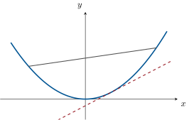
$f \colon I \to \R$ is convex when every chord lies above the graph:

\forall x, y \in I,\ \forall t \in \intcc{0}{1}, \quad f\bigl(tx + (1-t)y\bigr) \leq t f(x) + (1-t) f(y).

( $f$ is concave when $-f$ is convex.)

Theorem 14.19 (Differential characterizations)

Let $f$ be differentiable on $I$ . The following are equivalent:

$f$ is convex;
$f'$ is increasing on $I$ ;
the graph lies above every tangent: $f(y) \geq f(x) + f'(x)(y - x)$ for all $x, y \in I$ .

If $f$ is twice differentiable: $f$ convex $\iff f'' \geq 0$ .

Proof. (1 $\Rightarrow$ 3) Convexity written as $\frac{f(x + t(y-x)) - f(x)}{t} \leq f(y) - f(x)$ for $t \in \intoc{0}{1}$ ; let $t \to 0^+$ : $f'(x)(y - x) \leq f(y) - f(x)$ .

(3 $\Rightarrow$ 2) For $x < y$ , the two tangent inequalities at $x$ and at $y$ give $f'(x)(y-x) \leq f(y) - f(x) \leq f'(y)(y - x)$ , hence $f'(x) \leq f'(y)$ .

(2 $\Rightarrow$ 1) Fix $x < y$ and $t \in \intoo{0}{1}$ , and let $z = tx + (1-t)y \in \intoo{x}{y}$ . By the mean value theorem on $\intcc{x}{z}$ and $\intcc{z}{y}$ : there are $c_1 < z < c_2$ with

\frac{f(z) - f(x)}{z - x} = f'(c_1) \leq f'(c_2) = \frac{f(y) - f(z)}{y - z} ,

and clearing denominators ( $z - x = (1-t)(y-x)$ , $y - z = t(y-x)$ ) rearranges exactly into the convexity inequality.

Twice differentiable case: $f'' \geq 0 \iff f'$ increasing (Corollary 14.12). ∎

Convexity, twice: every chord (gray) lies above the graph, and the graph lies above every tangent (dashed).

Example 14.20 (Classical convexity inequalities)

$\exp$ is convex ( $\exp'' = \exp > 0$ ): its tangent at $0$ gives $\eu^x \geq 1 + x$ for all $x$ . $\ln$ is concave: its tangent at $1$ gives $\ln x \leq x - 1$ ; its chords give, for $0 < a \leq b$ , the inequality between geometric and arithmetic means: taking $t = \frac12$ in concavity,

\ln\frac{a + b}{2} \geq \frac{\ln a + \ln b}{2} = \ln\sqrt{ab}, \qquad\text{so}\qquad \sqrt{ab} \leq \frac{a+b}{2} .

The general arithmetic–geometric inequality is Exercise 14.9.

Example 14.21 (A convexity inequality from scratch)

The function $f(t) = t\ln t$ is convex on $\intoo{0}{+\infty}$ : $f''(t) = \frac1t > 0$ . Its midpoint inequality, multiplied by $2$ , reads: for all $a, b > 0$ ,

a\ln a + b\ln b \;\geq\; (a + b)\,\ln\frac{a + b}{2} ,

with equality iff $a = b$ (strict convexity). Test drive: $a = 1$ , $b = 3$ gives $3\ln 3 = 3.296$ against $4\ln 2 = 2.773$ . This innocuous inequality is the two-point case of the entropy comparison that reappears with Jensen’s inequality (Exercise 14.9) and in the information-theoretic asymptotics of the Year 3 volume. The closing insight: to manufacture an inequality, find a function whose second derivative has a sign and write down what convexity says — the differential characterization turns one sign check into infinitely many inequalities.

Remark 14.22 (Common pitfalls with derivatives)

(i) A positive derivative at one point does not give monotonicity near it: $f(x) = \frac x2 + x^2\sin\frac1x$ (with $f(0) = 0$ ) has $f'(0) = \frac12 > 0$ , yet

f'(x) = \frac12 + 2x\sin\frac1x - \cos\frac1x

equals $-\frac12$ at each $x_n = \frac{1}{2\pi n}$ : every neighborhood of $0$ contains descents. Monotonicity needs $f' \geq 0$ on an interval (Corollary 14.12); the pointwise sign only controls the crossing of the tangent line. (ii) Rolle’s three hypotheses are all active: $\abs x$ on $\intcc{-1}{1}$ (no interior differentiability), $x$ on $\intcc{0}{1}$ (ends not equal), and $x - \lfloor x\rfloor$ on $\intcc{0}{1}$ (continuity fails at $1$ ) each break exactly one hypothesis and the conclusion. (iii) Derivatives may be discontinuous, but not arbitrarily: $f'$ can oscillate (Example 14.2) yet always satisfies the intermediate value property (Darboux, Exercise 14.10): a derivative never jumps — if you compute a one-sided “derivative limit” with a jump, you have differentiated a non-differentiable function. (iv) The inverse formula needs $f' \neq 0$ : $x \mapsto x^3$ is a smooth strictly increasing bijection whose inverse $x^{1/3}$ has a vertical tangent at $0$ — differentiability of the inverse is lost exactly where $f'$ vanishes (Theorem 14.5).

Remark 14.23 (Where the mean value theorem works next)

Nearly every quantitative statement of the next chapters is this chapter’s mean value theorem in costume: the fundamental theorem of calculus (Chapter 15) differentiates the area function and concludes with the monotonicity criterion; the Taylor–Lagrange formula (Chapter 16) is the mean value theorem iterated $n$ times; the error analysis of Newton’s method and of fixed-point iterations (Exercise 14.11) is the Lipschitz form; and this chapter’s weekend problem (Problem 14.1) turns the same Lipschitz bound into number theory — a repulsion inequality between algebraic numbers and rationals, yielding the first transcendental number in history. In the Year 2 volume, the mean value inequality survives in several variables when the equality does not.

Example 14.24 (Young’s inequality from concavity)

Let $p, q > 1$ with $\frac1p + \frac1q = 1$ . For all $a, b > 0$ :

ab \;\leq\; \frac{a^p}{p} + \frac{b^q}{q} .

Proof by one application of the concavity of $\ln$ with weights $\frac1p, \frac1q$ (the two-point Jensen inequality, as in Exercise 14.9):

\ln\Bigl(\frac{a^p}{p} + \frac{b^q}{q}\Bigr) \;\geq\; \frac1p \ln(a^p) + \frac1q \ln(b^q) = \ln a + \ln b = \ln(ab),

and $\ln$ increasing converts the inequality of logarithms into the claim; equality iff $a^p = b^q$ (strict concavity). The case $p = q = 2$ is the arithmetic-geometric inequality $ab \leq \frac{a^2 + b^2}{2}$ in disguise. The closing insight: Young’s inequality is the algebraic seed of the Hölder and Minkowski inequalities of the Year 2 volume — one concavity statement about $\ln$ , harvested for norms.

Remark 14.25 (Perspectives inside this volume)

The derivative acquires three new lives before the volume ends. In Chapter 16 it iterates: $n$ derivatives at a point compress into one polynomial plus a controlled error, and the mean value theorem becomes the Lagrange remainder. In Chapter 24, differentiation turns geometric: for a parametrized curve $t \mapsto (x(t), y(t))$ , the pair $(x'(t), y'(t))$ is a velocity vector, tangency becomes collinearity, and critical points become cusps to classify. In Chapter 25, one variable is frozen at a time: partial derivatives repeat this chapter twice over, and the tangent line grows into a tangent plane. All three chapters inherit the same grammar — local linear approximation plus an error term — first spoken here.

14.4 Exercises

Exercise 14.1 ★

Differentiate (specifying the domains): $x^x$ ; $\;\ln\bigl(x + \sqrt{x^2+1}\bigr)$ ; $\;\arctan\frac{1}{x}$ ; $\;\sqrt{1 + \eu^{2x}}$ .

Solution

Solution of Exercise 14.1.

$x^x = \eu^{x\ln x}$ on $\intoo{0}{+\infty}$ : derivative $(\ln x + 1)\,x^x$ .

$\ln(x + \sqrt{x^2+1})$ on $\R$ (the argument is always $> 0$ ): derivative $\frac{1}{\sqrt{x^2+1}}$ (computed in Proposition 4.21 — it is $\operatorname{arsinh}$ ).

$\arctan\frac1x$ on $\R^*$ : derivative $\frac{-1/x^2}{1 + 1/x^2} = \frac{-1}{1 + x^2}$ (consistent with Proposition 4.12 (2): the function is $\pm\frac\pi2 - \arctan x$ on each half-line).

$\sqrt{1 + \eu^{2x}}$ on $\R$ : derivative $\frac{\eu^{2x}}{\sqrt{1 + \eu^{2x}}}$ .

Exercise 14.2 ★

Complete Example 14.2: prove that $f(x) = x^2 \sin\frac1x$ , $f(0) = 0$ , is differentiable at $0$ with $f'(0) = 0$ , and that $f'$ has no limit at $0$ .

Solution

Solution of Exercise 14.2.

At $0$ : $\bigl|\frac{f(h) - 0}{h}\bigr| = \abs{h \sin\frac1h} \leq \abs h \to 0$ , so $f'(0) = 0$ . For $x \neq 0$ , the usual rules give $f'(x) = 2x\sin\frac1x - \cos\frac1x$ . Along $x_n = \frac{1}{2\pi n}$ : $f'(x_n) = 0 - 1 \to -1$ ; along $y_n = \frac{1}{(2n+1)\pi}$ : $f'(y_n) = 0 + 1 \to 1$ . Two sequences tending to $0$ with different limits of $f'$ : no limit (Theorem 13.3), so $f'$ is not continuous at $0$ and $f$ is differentiable without being $C^1$ .

Exercise 14.3 ★

Using the mean value theorem or the tangent inequalities, prove that for all $x > 0$ :

\frac{x}{1 + x} < \ln(1 + x) < x .

Deduce $\lim_{n\to\infty} \bigl(1 + \frac xn\bigr)^n = \eu^x$ for every $x > 0$ .

Solution

Solution of Exercise 14.3.

$\ln(1+x) < x$ for $x > 0$ : concavity tangent inequality at $0$ (strict away from the contact point since $\ln$ is strictly concave; or apply the mean value theorem: $\ln(1+x) = \frac{x}{1+c}$ for some $c \in \intoo{0}{x}$ , and $\frac{x}{1+c} < x$ ). The same mean value identity gives the lower bound: $\frac{x}{1+c} > \frac{x}{1+x}$ .

Consequence: with $x/n$ in place of $x$ ,

\frac{x/n}{1 + x/n} < \ln\Bigl(1 + \frac xn\Bigr) < \frac xn \quad\implies\quad \frac{x}{1 + x/n} < n \ln\Bigl(1 + \frac xn\Bigr) < x .

The left member tends to $x$ : by the squeeze, $n\ln(1 + \frac xn) \to x$ , and by continuity of $\exp$ , $\bigl(1 + \frac xn\bigr)^n = \eu^{n\ln(1 + x/n)} \to \eu^x$ .

Exercise 14.4 ★

Let $P$ be a real polynomial with $k$ distinct real roots. Prove that $P'$ has at least $k - 1$ distinct real roots, interlaced with those of $P$ . Deduce that if $P$ has all its roots real, so does $P'$ .

Solution

Solution of Exercise 14.4.

Let $x_1 < x_2 < \dots < x_k$ be distinct roots of $P$ . On each $\intcc{x_i}{x_{i+1}}$ , Rolle (Theorem 14.8) produces $c_i \in \intoo{x_i}{x_{i+1}}$ with $P'(c_i) = 0$ : that is $k - 1$ roots of $P'$ , distinct because the open intervals are disjoint — and interlaced by construction.

If $P$ (degree $n$ ) has all roots real, write them with multiplicities $m_1 + \dots + m_k = n$ . Each root of multiplicity $m_i \geq 2$ is a root of $P'$ of multiplicity $m_i - 1$ (Proposition 8.11), contributing $\sum (m_i - 1) = n - k$ ; Rolle contributes $k - 1$ more, all distinct from these. Total $\geq n - 1 = \deg P'$ : all roots of $P'$ are real.

Exercise 14.5 ★★

Let $f$ be differentiable on $\R$ with $f' (x)\to \ell$ as $x \to +\infty$ . Prove that $\frac{f(x)}{x} \to \ell$ (mean value theorem on $\intcc{A}{x}$ ). Does $f(x+1) - f(x) \to \ell$ hold too?

Solution

Solution of Exercise 14.5.

Fix $\varepsilon > 0$ and $A$ with $\abs{f'(t) - \ell} \leq \varepsilon$ for $t \geq A$ . For $x > A$ , the mean value theorem on $\intcc{A}{x}$ gives $c \in \intoo{A}{x}$ with

f(x) = f(A) + f'(c)(x - A), \qquad\text{so}\qquad \Bigl|\frac{f(x)}{x} - \ell\Bigr| \leq \frac{\abs{f(A)} + \abs\ell A}{x} + \abs{f'(c) - \ell} \cdot\frac{x - A}{x} \leq \frac{C_A}{x} + \varepsilon .

For $x$ large, $\frac{C_A}{x} \leq \varepsilon$ : hence $\frac{f(x)}{x} \to \ell$ .

Yes: $f(x+1) - f(x) = f'(c_x)$ with $c_x \in \intoo{x}{x+1}$ (mean value theorem on $\intcc{x}{x+1}$ ), and $c_x \to +\infty$ , so $f(x+1) - f(x) \to \ell$ .

Exercise 14.6 ★★

(A discrete Rolle) Let $f$ be $n$ times differentiable on $I$ and vanish at $n + 1$ distinct points. Prove that $f^{(n)}$ vanishes at least once. Application: a polynomial of degree $\leq n$ vanishing at $n+1$ points is zero (again).

Solution

Solution of Exercise 14.6.

Induction on $n$ . For $n = 1$ : Rolle. If the claim holds for $n - 1$ : $f$ vanishes at $n+1$ points, so by Rolle applied on the $n$ gaps, $f'$ vanishes at $n$ distinct points; the induction hypothesis applied to $f'$ ( $n-1$ times differentiable, $n$ zeros) makes $(f')^{(n-1)} = f^{(n)}$ vanish somewhere.

Application: if $P$ of degree $\leq n$ vanishes at $n+1$ points, then $P^{(n)}$ , a constant equal to $n!$ times the leading coefficient, vanishes: the leading coefficient is $0$ , and one concludes by downward induction (or directly: all coefficients vanish).

Exercise 14.7 ★★

Let $f$ be twice differentiable on $\intcc{a}{b}$ with $f(a) = f(b) = 0$ and $f(x_0) > 0$ for some interior $x_0$ . Prove that $f''(c) < 0$ for some $c \in \intoo{a}{b}$ . (Two mean value theorems and a comparison of slopes.)

Solution

Solution of Exercise 14.7.

By the mean value theorem on $\intcc{a}{x_0}$ and on $\intcc{x_0}{b}$ :

f'(c_1) = \frac{f(x_0) - f(a)}{x_0 - a} = \frac{f(x_0)}{x_0 - a} > 0, \qquad f'(c_2) = \frac{f(b) - f(x_0)}{b - x_0} = \frac{-f(x_0)}{b - x_0} < 0,

with $c_1 < x_0 < c_2$ . Then the mean value theorem applied to $f'$ on $\intcc{c_1}{c_2}$ gives $c$ with

f''(c) = \frac{f'(c_2) - f'(c_1)}{c_2 - c_1} < 0 . \qedhere

Exercise 14.8 ★★

Study the function $f(x) = \dfrac{\ln x}{x}$ on $\intoo{0}{+\infty}$ : variations, limits, maximum. Deduce that $a^b > b^a$ for all reals $\eu \leq a < b$ , and settle the famous special case: which of $\eu^\pi$ , $\pi^\eu$ is larger? Check against the small integer pairs $(2,3)$ and $(2,4)$ : why do they behave differently?

Solution

Solution of Exercise 14.8.

$f'(x) = \frac{1 - \ln x}{x^2}$ : $f$ increases on $\intoc{0}{\eu}$ , decreases on $\intco{\eu}{+\infty}$ , with maximum $f(\eu) = \frac1\eu$ ; limits $-\infty$ at $0^+$ and $0$ at $+\infty$ (growth comparison).

For $\eu \leq a < b$ : $f$ strictly decreasing there gives $\frac{\ln a}{a} > \frac{\ln b}{b}$ , i.e. $b \ln a > a \ln b$ , i.e. $a^b > b^a$ .

With $a = \eu < b = \pi$ : $\eu^\pi > \pi^\eu$ .

Small pairs: $(2, 3)$ : $2^3 = 8 < 9 = 3^2$ — reversed! The reason: $2 < \eu$ , and on $\intoo{0}{\eu}$ the function $f$ is increasing, so the comparison flips when both numbers sit below $\eu$ , and is unpredictable across $\eu$ ( $f(2) = f(4)$ explains the tie $2^4 = 4^2 = 16$ ).

Exercise 14.9 ★★

(Arithmetic–geometric inequality) Using the concavity of $\ln$ with general weights (Jensen’s inequality for $n$ points, to be proved by induction on $n$ ), show that for positive reals $a_1, \dots, a_n$ :

\sqrt[n]{a_1 a_2 \cdots a_n} \leq \frac{a_1 + \dots + a_n}{n},

with equality iff all $a_i$ are equal.

Solution

Solution of Exercise 14.9.

Jensen for $\ln$ , by induction on $n$ . Claim: for positive $x_i$ and weights $\lambda_i > 0$ with $\sum \lambda_i = 1$ : $\ln\bigl(\sum \lambda_i x_i\bigr) \geq \sum \lambda_i \ln x_i$ . For $n = 2$ this is concavity. Step: with $\Lambda = \lambda_1 + \dots + \lambda_{n-1} = 1 - \lambda_n$ and $y = \sum_{i<n} \frac{\lambda_i}{\Lambda} x_i$ ,

\ln\Bigl(\sum_{i \leq n} \lambda_i x_i\Bigr) = \ln\bigl(\Lambda y + \lambda_n x_n\bigr) \geq \Lambda \ln y + \lambda_n \ln x_n \geq \Lambda \sum_{i<n} \frac{\lambda_i}{\Lambda}\ln x_i + \lambda_n \ln x_n,

using concavity ( $n = 2$ ) then the induction hypothesis.

With $\lambda_i = \frac 1n$ and $x_i = a_i$ : $\ln\frac{\sum a_i}{n} \geq \frac 1n \sum \ln a_i = \ln\sqrt[n]{a_1\cdots a_n}$ ; exponentiate. Equality: $\ln$ is strictly concave ( $\ln'' < 0$ ), so equality at each step forces the averaged points to coincide — i.e. all $a_i$ equal; and if all are equal, equality is clear.

Exercise 14.10 ★★★

(Darboux: derivatives take intermediate values) Let $f$ be differentiable on $I$ and $a < b$ in $I$ with $f'(a) < v < f'(b)$ . By considering $g(x) = f(x) - vx$ and the point where $g$ attains its minimum on $\intcc{a}{b}$ , prove that $f'(c) = v$ for some $c \in \intoo{a}{b}$ — even though $f'$ need not be continuous (Exercise 14.2).

Solution

Solution of Exercise 14.10.

Let $g(x) = f(x) - vx$ : differentiable, with $g'(a) = f'(a) - v < 0$ and $g'(b) = f'(b) - v > 0$ . By the extreme value theorem, $g$ attains its minimum on $\intcc{a}{b}$ at some $c$ . It is not at $a$ : since $g'(a) < 0$ , points just right of $a$ have $g < g(a)$ . It is not at $b$ : since $g'(b) > 0$ , points just left of $b$ have $g < g(b)$ . So $c$ is interior, and Proposition 14.7 gives $g'(c) = 0$ , i.e. $f'(c) = v$ .

Exercise 14.11 ★★★

Let $f \colon \R \to \R$ be differentiable with $\abs{f'(x)} \leq k < 1$ for all $x$ (a contraction). Prove that $f$ has exactly one fixed point $\ell$ , and that every sequence $u_{n+1} = f(u_n)$ converges to $\ell$ with $\abs{u_n - \ell} \leq k^n\abs{u_0 - \ell}$ . (Existence: apply the intermediate value theorem to $f(x) - x$ on a large segment, using the Lipschitz bound; or use completeness with the Cauchy criterion.)

Solution

Solution of Exercise 14.11.

Uniqueness: two fixed points $\ell \neq \ell'$ would give $\abs{\ell - \ell'} = \abs{f(\ell) - f(\ell')} \leq k\abs{\ell - \ell'} < \abs{\ell - \ell'}$ , absurd.

Existence: $g(x) = f(x) - x$ satisfies, by the mean value inequality, $f(x) \leq f(0) + k\abs x$ ; so for $x \geq \frac{\abs{f(0)}}{1 - k}$ , $g(x) \leq f(0) + kx - x \leq 0$ , and symmetrically $g(-x) \geq 0$ for $x$ large. The intermediate value theorem gives a zero $\ell$ of $g$ : a fixed point.

Convergence: the mean value inequality again:

\abs{u_{n+1} - \ell} = \abs{f(u_n) - f(\ell)} \leq k\abs{u_n - \ell},

so by induction $\abs{u_n - \ell} \leq k^n \abs{u_0 - \ell} \to 0$ .

Exercise 14.12 ★★★

(Cauchy’s mean value theorem and l’Hospital’s rule)

Let $f, g$ be continuous on $\intcc{a}{b}$ , differentiable on $\intoo{a}{b}$ , with $g'$ never zero there. Prove that $g(b) \neq g(a)$ and that some $c \in \intoo{a}{b}$ satisfies

$\frac{f(b) - f(a)}{g(b) - g(a)} = \frac{f'(c)}{g'(c)}$

(apply Rolle to $h = f - \lambda g$ for the right constant $\lambda$ ).
Deduce l’Hospital’s rule in the $\frac00$ form at a point: if $f(a) = g(a) = 0$ and $\frac{f'(x)}{g'(x)} \to \ell$ as $x \to a^+$ , then $\frac{f(x)}{g(x)} \to \ell$ .
Show the converse fails: for $f(x) = x^2\sin\frac1x$ ( $f(0) = 0$ ) and $g(x) = x$ , the quotient $\frac{f}{g}$ has a limit at $0$ but $\frac{f'}{g'}$ has none.

Solution

Solution of Exercise 14.12.

If $g(b) = g(a)$ , Rolle would give an interior zero of $g'$ : excluded. Set $\lambda = \frac{f(b) - f(a)}{g(b) - g(a)}$ and $h = f - \lambda g$ : $h$ is continuous on $\intcc{a}{b}$ , differentiable inside, and $h(b) - h(a) = f(b) - f(a) - \lambda(g(b) - g(a)) = 0$ . Rolle provides $c$ with $h'(c) = 0$ , i.e. $f'(c) = \lambda\,g'(c)$ ; divide by $g'(c) \neq 0$ .
For $x > a$ close to $a$ , part (1) on $\intcc{a}{x}$ (where $g' \neq 0$ ) gives $g(x) \neq 0$ and $c_x \in \intoo{a}{x}$ with

$\frac{f(x)}{g(x)} = \frac{f(x) - f(a)}{g(x) - g(a)} = \frac{f'(c_x)}{g'(c_x)} .$

As $x \to a^+$ , $c_x \to a^+$ (squeeze), so the right side tends to $\ell$ : $\frac{f}{g} \to \ell$ .
$\frac{f(x)}{g(x)} = x\sin\frac1x \to 0$ , while $\frac{f'(x)}{g'(x)} = 2x\sin\frac1x - \cos\frac1x$ has no limit at $0$ (Exercise 14.2): l’Hospital’s rule transfers information only from $\frac{f'}{g'}$ to $\frac fg$ , never back.

14.5 Problem: Liouville’s inequality and the first transcendental number

Problem 14.1

Weekend problem — algebraic numbers repel rationals: $\abs{x - p/q} \geq C/q^d$ , and the transcendence of $\sum 10^{-n!}$

A real number is algebraic when it is a root of a nonzero polynomial with integer coefficients, and transcendental otherwise. In 1844 Liouville produced the first number ever proved transcendental, and the engine of his proof is this chapter’s mean value theorem: an algebraic number of degree $d$ cannot be approximated by rationals better than $C/q^d$ — so a number approximable faster than every power cannot be algebraic. This problem builds the inequality, constructs Liouville’s number $L = 0.110001000\dots$ (ones at the factorial positions, via the digit machinery of Problem 10.1), proves its transcendence, and ends with Cantor’s rival proof and effective bounds for $\sqrt2$ and $2^{1/3}$ .

Part I — How well can rationals be approximated?

Show that two distinct rationals $\frac ab \neq \frac pq$ (written with $b, q \geq 1$ ) satisfy $\bigl|\frac ab - \frac pq\bigr| \geq \frac{1}{bq}$ . Deduce: if $x = \frac ab$ and $0 < \bigl|x - \frac pq\bigr| < \frac{1}{bq}$ , no such $\frac pq$ exists — a rational repels all other rationals at scale $\frac 1q$ .
Prove that for every rational $\frac pq$ ( $q \geq 1$ ): $\bigl|\sqrt2 - \frac pq\bigr| \geq \frac{1}{4q^2}$ (if the distance exceeds $1$ this is clear; otherwise bound $\abs{\sqrt2 + p/q} < 4$ and use the nonzero integer $\abs{p^2 - 2q^2} \geq 1$ ).
In the other direction: check that $(p, q) \mapsto (p + 2q, p + q)$ preserves $\abs{p^2 - 2q^2} = 1$ , generate from $(1,1)$ the pairs $(3,2)$ , $(7,5)$ , $(17,12)$ , $(41,29)$ , $(99,70)$ , and show each satisfies

$\Bigl|\sqrt2 - \frac pq\Bigr| = \frac{1}{q^2\,(\sqrt2 + p/q)} < \frac{1}{2q^2} :$

infinitely many approximations of order $2$ . With question 2: the approximation exponent of $\sqrt 2$ is exactly $2$ .
(Dirichlet) Let $x$ be irrational and $N \in \N^*$ . Consider the $N + 1$ fractional parts of $0, x, 2x, \dots, Nx$ in the $N$ boxes $\intco{\frac kN}{\frac{k + 1}{N}}$ : by the pigeonhole principle (Corollary 2.3), two fall in one box. Deduce $q \leq N$ and $p$ with $\abs{qx - p} < \frac 1N$ , hence infinitely many rationals with $\bigl|x - \frac pq\bigr| < \frac{1}{q^2}$ : every irrational is approximable to order $2$ .

Part II — Liouville’s inequality. Let $x$ be irrational and algebraic.

Show that among the nonzero integer polynomials vanishing at $x$ there is one, say $P$ of degree $d$ , with no rational root; and check $d \geq 2$ (divide out a factor $X - \frac ab$ over $\Q$ and clear denominators; degree $1$ would make $x$ rational).
Show that for every rational $\frac pq$ ( $q \geq 1$ ): $\bigl|P\bigl(\frac pq\bigr)\bigr| \geq \frac{1}{q^d}$ ( $q^d P(p/q)$ is a nonzero integer).
Let $M = \max_{\intcc{x-1}{x+1}} \abs{P'}$ (Theorem 13.13). Using the mean value theorem between $x$ and $\frac pq$ , prove Liouville’s inequality: with $C = \min\bigl(1, \frac 1M\bigr) > 0$ ,

$\Bigl| x - \frac pq \Bigr| \geq \frac{C}{q^{\,d}} \qquad\text{for every rational } \frac pq,\ q \geq 1 .$
Call $x$ a Liouville number when for every $n \in \N$ there is a rational $\frac pq$ with $q \geq 2$ and $0 < \bigl|x - \frac pq\bigr| < q^{-n}$ . Prove that a Liouville number is irrational (question 1: choose $n$ with $2^{\,n-1} > b$ ).
Prove Liouville’s theorem: a Liouville number is transcendental (combine questions 7 and 8: the inequality $C < q^{\,d-n}$ fails for large $n$ ).

Part III — The number $L$ .

Let $L$ be the value (in the sense of Problem 10.1) of the decimal digit string with digit $1$ at the positions $n!$ ( $n = 1, 2, 3, \dots$ ) and $0$ elsewhere, i.e. $L = \sup_k t_k$ with $t_k = \sum_{n=1}^{k} 10^{-n!}$ . Write out the first $25$ digits of $L$ .
Prove the tail bracketing, for every $k \geq 1$ :

$10^{-(k+1)!} \;\leq\; L - t_k \;\leq\; \frac{10}{9}\,10^{-(k+1)!} \;<\; 2\cdot 10^{-(k+1)!}$

(bound every partial sum beyond $t_k$ by a finite geometric sum).
Write $t_k = \frac{p_k}{q_k}$ with $q_k = 10^{k!}$ . Show $0 < L - \frac{p_k}{q_k} < \frac{2}{q_k^{\,k+1}}$ , and conclude that $L$ is a Liouville number in the sense of question 8.
Conclude: $L$ is transcendental — the first explicit example in history (Liouville, 1844). Cross-check its irrationality directly: its digits are not eventually periodic (growing gaps, as in Problem 10.1, question 20).
Generalize: replace each digit $1$ by an arbitrary nonzero digit $d_n \in \intint{1}{9}$ . Show the value is still a Liouville number, and deduce — by the diagonal argument of Problem 10.1 (question 22) applied to these digit choices — that there are uncountably many transcendental numbers of this shape.

Part IV — The hierarchy of approximation orders. Say $x$ is approximable to order $\mu$ when for some constant $c > 0$ infinitely many rationals satisfy $\bigl|x - \frac pq\bigr| < \frac{c}{q^{\mu}}$ .

Assemble the hierarchy from Parts I–III: rationals are approximable to order $1$ and no better; $\sqrt 2$ to order $2$ and no better; every irrational to order at least $2$ ; an algebraic number of degree $d$ to no order beyond $d$ ; Liouville numbers to every order. Justify each claim by citing the relevant question.
Show that $L + r$ is a Liouville number for every rational $r = \frac ab$ (translate the approximants: the new denominators are $b\,q_k$ ). Conclude that Liouville — hence transcendental — numbers are dense in $\R$ .
(Cantor, 1874) Prove that the set of algebraic numbers is countable: there are finitely many integer polynomials with degree plus sum of $\abs{\text{coefficients}}$ bounded by $h$ , each with at most $\deg$ roots; a countable union of finite sets is countable. Since no sequence exhausts $\R$ (Problem 10.1, question 22), transcendental numbers exist — in fact form an uncountable set. Compare the two proofs: what does Liouville’s give that Cantor’s cannot?
Prove directly from question 2 that $\sqrt 2$ is not a Liouville number (for $n \geq 3$ , the inequality $q^{-n} > \frac{1}{4q^2}$ bounds $q$ ; then only finitely many candidate rationals remain, all at positive distance from $\sqrt2$ ). Generalize: no algebraic number is Liouville.

Part V — Effective constants.

For the Pell pair $(99, 70)$ : verify $99^2 - 2\cdot70^2 = 1$ and evaluate the exact error

$\sqrt2 - \frac{99}{70} = \frac{-1}{70^2\,\bigl(\sqrt2 + \frac{99}{70}\bigr)}, \qquad \Bigl|\sqrt 2 - \frac{99}{70}\Bigr| \approx 7.2\cdot 10^{-5} :$

five correct digits from a three-digit fraction.
Run Part II on $x = 2^{1/3}$ , $P = X^3 - 2$ : check $P$ has no rational root, bound $M = \max_{\intcc{x-1}{x+1}} 3t^2 \leq 3\,(1 + 2^{1/3})^2 < 16$ , and conclude the effective inequality

$\Bigl| 2^{1/3} - \frac pq \Bigr| \geq \frac{1}{16\,q^3} \qquad \text{for all } \frac pq .$
Payoff: show that any rational approximating $2^{1/3}$ within $10^{-6}$ must have denominator $q \geq 40$ .
Show that the base $10$ is irrelevant: the binary analogue $\sum_{n\geq1} 2^{-n!}$ (value of the binary string with ones at factorial positions) is also a Liouville number, hence transcendental.

Part VI — Frontiers and synthesis.

Let $x^\dagger$ be the value of the decimal string with ones exactly at the positions $3^k$ ( $k \geq 0$ ). Show $x^\dagger$ is approximable to order $3$ , and deduce from Liouville’s inequality that $x^\dagger$ is neither rational nor a quadratic irrational. Explain why the method stalls there: order $3$ is compatible with algebraicity of degree $\geq 3$ , and closing that gap (any exponent $> 2$ suffices, for every algebraic number) is Roth’s theorem, far beyond this volume.
Quantify Cantor: show that the algebraic numbers of degree $\leq d$ given by polynomials with coefficients in $\intint{-H}{H}$ number at most $d\,(2H + 1)^{d+1}$ . (This finiteness is what made question 17 work.)
Synthesis, one sentence each: (i) locate the single analytic ingredient of Liouville’s proof (which theorem of this chapter, used where); (ii) state the tension that powers it (integrality forces $\abs{P(p/q)} \geq q^{-d}$ , smoothness forbids $\abs{P(p/q)} > M\abs{x - p/q}$ ); (iii) contrast Liouville’s and Cantor’s proofs of the existence of transcendental numbers; (iv) name where this volume meets the theme again — the weekend problem of Chapter 15 proves $\pi$ irrational by the same integrality-versus-smallness squeeze, with integrals in place of derivatives.

Solution

Solution of Problem 14.1.

1. $\bigl|\frac ab - \frac pq\bigr| = \frac{\abs{aq - bp}}{bq}$ , and $aq - bp$ is a nonzero integer when the fractions differ: the distance is $\geq \frac{1}{bq}$ . So no rational other than $x$ itself enters the punctured interval of radius $\frac{1}{bq}$ around $x = \frac ab$ .

2. If $\bigl|\sqrt2 - \frac pq\bigr| \geq 1 \geq \frac{1}{4q^2}$ , done. Otherwise $\frac pq \in \intoo{\sqrt2 - 1}{\sqrt2 + 1}$ , so $0 < \sqrt2 + \frac pq < 2\sqrt2 + 1 < 4$ . Since $\sqrt 2 \notin \Q$ , $p^2 - 2q^2$ is a nonzero integer, and

\Bigl|\sqrt2 - \frac pq\Bigr| = \frac{\abs{2q^2 - p^2}}{q^2\,\bigl(\sqrt2 + \frac pq\bigr)} \geq \frac{1}{4q^2} .

3. $(p + 2q)^2 - 2(p + q)^2 = -(p^2 - 2q^2)$ : the value $\pm1$ propagates. From $(1,1)$ :

(3,2),\ (7,5),\ (17,12),\ (41,29),\ (99,70),

with $p^2 - 2q^2$ alternating $-1, +1, \dots$ For these, $\frac pq \geq 1$ , so $\sqrt2 + \frac pq > 2$ and

\Bigl|\sqrt2 - \frac pq\Bigr| = \frac{1}{q^2(\sqrt2 + p/q)} < \frac{1}{2q^2} ,

with $q \to \infty$ : infinitely many order- $2$ approximations. With question 2, the exponent $2$ is exact for $\sqrt 2$ .

4. The $N + 1$ numbers $kx - \lfloor kx\rfloor$ ( $0 \leq k \leq N$ ) lie in the $N$ boxes $\intco{\frac jN}{\frac{j+1}{N}}$ : two share a box (Corollary 2.3), say for $i < j$ . With $q = j - i \leq N$ and $p = \lfloor jx\rfloor - \lfloor ix\rfloor$ : $\abs{qx - p} < \frac1N$ , so $\bigl|x - \frac pq\bigr| < \frac{1}{Nq} \leq \frac{1}{q^2}$ . Letting $N \to \infty$ : since $x$ is irrational, each fixed fraction has positive distance to $x$ , while $\frac{1}{Nq} \leq \frac 1N \to 0$ forces new fractions to appear: infinitely many distinct $\frac pq$ with $\bigl|x - \frac pq\bigr| < \frac{1}{q^2}$ .

5. Start from any nonzero integer $P_0$ with $P_0(x) = 0$ . If $P_0$ has a rational root $\frac ab$ , the factor theorem (Theorem 8.7) writes $P_0 = \bigl(X - \frac ab\bigr)Q$ with $Q \in \Q[X]$ ; since $x \neq \frac ab$ ( $x$ irrational), $Q(x) = 0$ , and clearing denominators gives a nonzero integer polynomial of smaller degree vanishing at $x$ . The degree drops at each step, so the process stops: we reach $P \in \Z[X]$ , $P(x) = 0$ , with no rational root, of some degree $d$ . If $d \leq 1$ , $P = uX + v$ would make $x = -\frac vu$ rational: so $d \geq 2$ .

6. $q^d\,P\bigl(\frac pq\bigr) = a_d p^d + a_{d-1} p^{d-1} q + \dots + a_0 q^d$ is an integer, and it is nonzero because $P$ has no rational root: $\bigl|P\bigl(\frac pq\bigr)\bigr| \geq q^{-d}$ .

7. Note $M > 0$ : $P'$ is a nonzero polynomial ( $d \geq 2$ ), so it cannot vanish identically on $\intcc{x-1}{x+1}$ . If $\bigl|x - \frac pq\bigr| > 1$ , then it exceeds $\frac{C}{q^d}$ trivially. Otherwise $\frac pq \in \intcc{x-1}{x+1}$ and the mean value theorem (Theorem 14.9) gives $c$ between $x$ and $\frac pq$ with

\Bigl|P\Bigl(\frac pq\Bigr)\Bigr| = \Bigl|P\Bigl(\frac pq\Bigr) - P(x)\Bigr| = \abs{P'(c)}\,\Bigl|x - \frac pq\Bigr| \leq M\,\Bigl|x - \frac pq\Bigr| ,

so with question 6: $\bigl|x - \frac pq\bigr| \geq \frac{1}{Mq^d} \geq \frac{C}{q^d}$ .

8. Suppose $x = \frac ab$ is Liouville. Pick $n$ with $2^{n-1} > b$ and the corresponding $\frac pq$ , $q \geq 2$ :

0 < \Bigl|x - \frac pq\Bigr| < \frac{1}{q^n} = \frac{1}{q^{n-1}\,q} \leq \frac{1}{2^{n-1} q} < \frac{1}{bq} ,

contradicting question 1. So Liouville numbers are irrational.

9. If a Liouville $x$ were algebraic: it is irrational (question 8), so questions 5–7 provide $d \geq 2$ and $C > 0$ with $\bigl|x - \frac pq\bigr| \geq \frac{C}{q^d}$ always. For each $n$ , the Liouville approximant gives $\frac{C}{q^d} < q^{-n}$ , i.e. $C < q^{d-n} \leq 2^{d-n}$ (as $q \geq 2$ ). For $n$ large, $2^{d-n} < C$ : contradiction. Liouville numbers are transcendental.

10. Ones at positions $1, 2, 6, 24$ ; all other digits among the first $25$ vanish:

L = 0.1100010000\,0000000000\,00010\dots

11. For $m > k$ , the positions $n!$ with $n > k$ are distinct integers $\geq (k+1)!$ , so the finite geometric sum gives

t_m - t_k = \sum_{n=k+1}^{m} 10^{-n!} \leq \sum_{j = (k+1)!}^{m!} 10^{-j} < 10^{-(k+1)!}\,\frac{1}{1 - \frac1{10}} = \frac{10}{9}\,10^{-(k+1)!} ;

taking the supremum over $m$ : $L - t_k \leq \frac{10}{9}10^{-(k+1)!} < 2\cdot10^{-(k+1)!}$ . Lower bound: $L \geq t_{k+1} = t_k + 10^{-(k+1)!}$ .

12. $p_k = 10^{k!}\,t_k \in \N$ , $q_k = 10^{k!}$ , and $(k+1)! = (k+1)\,k!$ gives $10^{-(k+1)!} = q_k^{-(k+1)}$ : question 11 reads

0 < L - \frac{p_k}{q_k} < \frac{2}{q_k^{\,k+1}} .

Given $n$ : for $k \geq n$ , $2\,q_k^{-(k+1)} \leq q_k^{-n}$ (indeed $q_k^{\,k+1-n} \geq q_k \geq 10 > 2$ ), and $q_k \geq 2$ : the definition of question 8 is met. $L$ is a Liouville number.

13. By question 9, $L$ is transcendental — the first number in history proved transcendental (Liouville, 1844). Digit cross-check: the string has infinitely many ones with consecutive gaps $(k+1)! - k! = k\cdot k! \to \infty$ , so it is not eventually periodic, and $L \notin \Q$ by the periodicity criterion of Problem 10.1 (question 18) — consistent.

14. With digits $d_n \in \intint{1}{9}$ at the factorial positions: the tail bound of question 11 scales by at most $9$ : $0 < L' - t'_k \leq 9\cdot\frac{10}{9}\,10^{-(k+1)!} = 10\,q_k^{-(k+1)}$ (positivity because the digit at position $(k+1)!$ is nonzero). For $k \geq n$ : $10\,q_k^{-(k+1)} \leq q_k^{-n}$ since $q_k^{\,k+1-n} \geq 10$ : again a Liouville number, hence transcendental. These values are pairwise distinct for distinct digit choices (the strings are proper — zeros abound — and proper strings determine their value, Problem 10.1, question 10). Given any list $k \mapsto x_k$ of them, choose the $k$ -th factorial digit in $\intint{1}{9}$ different from that of $x_k$ : a number of the same shape missing from the list. Uncountably many explicit transcendentals.

15. First a lemma: if $\bigl|x - \frac pq\bigr| \geq \frac{C}{q^s}$ for all $\frac pq \neq x$ , then $x$ is not approximable to any order $\mu > s$ . Indeed infinitely many $\frac pq \neq x$ with $\bigl|x - \frac pq\bigr| < \frac{c}{q^\mu}$ would force $\frac{C}{q^s} < \frac{c}{q^\mu}$ , i.e. $q^{\mu - s} < \frac cC$ : the $q$ are bounded, and boundedly many fractions lie within distance $1$ of $x$ — finitely many candidates, not infinitely many. Now the hierarchy: rationals are approximable to order $1$ ( $\frac pq$ with $p = \lfloor qx\rfloor + 1$ gives error $\leq \frac1q < \frac2q$ ) and to no order $\mu > 1$ (question 1 gives the hypothesis of the lemma with $s = 1$ , $C = \frac1b$ ); $\sqrt2$ : order $2$ (question 3) and no more (question 2 and the lemma); every irrational: at least $2$ (question 4); algebraic of degree $d$ : at most $d$ (question 7 and the lemma); Liouville numbers: every order (question 12’s display, with $c = 2$ ).

16. With $r = \frac ab$ : $\frac{p_k}{q_k} + \frac ab = \frac{b p_k + a q_k}{b q_k} =: \frac{P_k}{Q_k}$ , $Q_k = b q_k \geq 2$ , and

\Bigl|(L + r) - \frac{P_k}{Q_k}\Bigr| = L - \frac{p_k}{q_k} < 2\,q_k^{-(k+1)} = 2\,b^{\,k+1} Q_k^{-(k+1)} .

Given $n$ : for large $k$ , $Q_k^{\,k+1-n} \geq Q_k = b\,10^{k!} \geq 2\,b^{\,k+1}$ (the factorial crushes the power), so the error is $< Q_k^{-n}$ : $L + r$ is Liouville. Since $\Q$ is dense and each $L + r$ is transcendental, transcendental numbers are dense in $\R$ .

17. For $h \geq 1$ there are finitely many $P \in \Z[X]$ with $\deg P + \sum_i \abs{a_i} \leq h$ (degree $\leq h$ and each coefficient in $\intint{-h}{h}$ : at most $(2h+1)^{h+1}$ ). Every nonzero integer polynomial has such a height, and has at most $\deg P$ real roots: the algebraic numbers form a countable union (over $h$ ) of finite sets, hence can be listed as a single sequence. If the transcendentals could also be listed, interleaving the two lists would list $\R$ , contradicting Problem 10.1 (question 22). So transcendental numbers form an uncountable set. Comparison: Cantor proves most reals are transcendental yet exhibits none; Liouville exhibits one, with effective constants (Part V) — existence by abundance versus existence by construction.

18. From question 2, the lemma hypothesis holds with $s = 2$ , $C = \frac14$ . If $\sqrt2$ were Liouville, then for $n = 3$ : $\frac{1}{4q^2} < q^{-3}$ forces $q < 4$ , so $q \in \{2, 3\}$ ; only finitely many $\frac pq$ with these $q$ lie within $1$ of $\sqrt2$ , each at some positive distance $\geq \varepsilon_0$ ( $\sqrt2$ irrational); choosing $n$ with $2^{-n} < \varepsilon_0$ leaves no admissible $\frac pq$ at all: contradiction. The same argument with $\frac{C}{q^d}$ shows no algebraic number is Liouville — question 9 in effective clothing.

19. $99^2 - 2\cdot70^2 = 9801 - 9800 = 1$ . Hence

\sqrt2 - \frac{99}{70} = \frac{2 - (99/70)^2}{\sqrt2 + 99/70} = \frac{-1}{4900\,\bigl(\sqrt2 + \tfrac{99}{70}\bigr)} , \qquad \Bigl|\sqrt2 - \frac{99}{70}\Bigr| = \frac{1}{4900 \times 2.8284\dots} \approx 7.2\cdot10^{-5} :

$\frac{99}{70} = 1.414285\dots$ against $\sqrt2 = 1.414213\dots$ — five correct digits.

20. Rational-root test for $P = X^3 - 2$ : candidates $\pm1, \pm2, \pm\frac12$ , none a root. So $d = 3$ and Part II applies to $x = 2^{1/3} = 1.2599\dots$ On $\intcc{x - 1}{x + 1} \subseteq \intcc{0.25}{2.26}$ : $\abs{P'(t)} = 3t^2 \leq 3\,(1 + 2^{1/3})^2 < 3\times(2.26)^2 = 15.32 < 16$ , so $M < 16$ and $C \geq \frac{1}{16}$ :

\Bigl|2^{1/3} - \frac pq\Bigr| \geq \frac{1}{16\,q^3} \qquad\text{for all rationals.}

21. If $\bigl|2^{1/3} - \frac pq\bigr| < 10^{-6}$ , then $\frac{1}{16 q^3} < 10^{-6}$ , i.e. $q^3 > \frac{10^6}{16} = 62\,500$ ; since $39^3 = 59\,319 < 62\,500 \leq 64\,000 = 40^3$ : $q \geq 40$ .

22. Run Part III in base $2$ : $B = \sup_k \sum_{n\leq k} 2^{-n!}$ , $q_k = 2^{k!}$ , and the geometric tail (ratio $\frac12$ ) gives $0 < B - \frac{p_k}{q_k} \leq 2\cdot2^{-(k+1)!} = 2\,q_k^{-(k+1)} \leq q_k^{-n}$ for $k \geq n$ . So $B$ is Liouville, hence transcendental: nothing in the argument is decimal.

23. With ones at positions $3^k$ : $q_k = 10^{3^k}$ and the tail bound gives $0 < x^\dagger - \frac{p_k}{q_k} < 2\cdot10^{-3^{k+1}} = 2\,q_k^{-3}$ (as $3^{k+1} = 3\cdot3^k$ ): infinitely many approximations of order $3$ . By the lemma of question 15: order $3 > 1$ rules out rationality, and order $3 > 2$ rules out being a quadratic irrational (whose Liouville inequality has $s = d = 2$ ). But an algebraic number of degree $\geq 3$ is only repelled at order $d \geq 3$ : Liouville’s method cannot separate $x^\dagger$ from the cubics. The gap is closed by Roth’s theorem — every algebraic irrational has approximation order exactly $2$ — a twentieth-century result far beyond this volume; granted it, $x^\dagger$ too is transcendental.

24. There are at most $(2H+1)^{d+1}$ tuples $(a_0, \dots, a_d)$ with entries in $\intint{-H}{H}$ , and each nonzero polynomial among them has at most $d$ real roots: at most $d\,(2H+1)^{d+1}$ algebraic numbers arise — the finiteness that let question 17 enumerate them all.

25. (i) The single analytic ingredient is the mean value theorem, in question 7, converting the vanishing $P(x) = 0$ into the Lipschitz repulsion $\abs{P(p/q)} \leq M\abs{x - p/q}$ . (ii) The tension: integrality pushes $\abs{P(p/q)}$ up to $q^{-d}$ , smoothness pulls it down to $M\abs{x - p/q}$ — a rational too close to $x$ would be crushed between the two. (iii) Liouville constructs one transcendental with effective constants; Cantor shows almost all reals are transcendental without naming one: construction versus cardinality. (iv) The weekend problem of Chapter 15 proves the irrationality of $\pi$ by the same squeeze — an integral that would be a positive integer yet is trapped in $\intoo{0}{1}$ — with integration replacing differentiation as the analytic half.