University Mathematics — Year 1 · Bachelor Year 1

13Limits and Continuity

The intermediate value theorem and the extreme value theorem were used at High School level on visual faith. With sequences (Chapter 11) and the topology of $\R$ (Chapter 12) in hand, this chapter proves them — and completes the theory with the monotone bijection theorem (which legitimizes $\arcsin$ , $\operatorname{arcosh}$ and their kin from Chapter 4) and Heine’s theorem on uniform continuity.

Throughout, $I$ is an interval and $f \colon I \to \R$ ; “ $x_0 \in \overline I$ ” allows limits at endpoints.

13.1 Limits of functions

Definition 13.1 (Limit at a point)

Let $x_0 \in \overline{I}$ and $\ell \in \R$ . Then $f(x) \to \ell$ as $x \to x_0$ when

\forall \varepsilon > 0,\ \exists \delta > 0,\ \forall x \in I, \qquad \abs{x - x_0} \leq \delta \implies \abs{f(x) - \ell} \leq \varepsilon .

Limits at $\pm\infty$ and infinite limits are defined by the same pattern ( $\abs{x - x_0} \leq \delta$ becomes $x \geq M$ ; $\abs{f(x) - \ell} \leq \varepsilon$ becomes $f(x) \geq M'$ ). One-sided limits restrict $x$ to $x > x_0$ (written $x \to x_0^+$ ) or $x < x_0$ . The limit is unique when it exists (same proof as Proposition 11.4).

Example 13.2 (A limit through the squeeze)

Compute $\lim_{x \to 0} x\,\bigl\lfloor \frac1x \bigr\rfloor$ . The floor bracketing $\frac1x - 1 < \lfloor \frac1x \rfloor \leq \frac1x$ gives, after multiplying by $x$ (mind the sign!):

1 - x < x\Bigl\lfloor \frac1x \Bigr\rfloor \leq 1 \quad (x > 0), \qquad 1 \leq x\Bigl\lfloor \frac1x \Bigr\rfloor < 1 - x \quad (x < 0),

and both one-sided squeezes close on $1$ : the limit is $1$ . Note what happened: $\lfloor \frac1x\rfloor$ alone has wild jumps near $0$ , but the factor $x$ tames each jump ( $x$ times a unit jump is small), and only the bracketing survives. The closing insight: limits of products of a small factor with a bounded-oscillation factor are squeeze problems, never operation-theorem problems — the operations theorem needs both factors to converge.

Theorem 13.3 (Sequential characterization)

$f(x) \to \ell$ as $x \to x_0$ if and only if: for every sequence $(u_n)$ of points of $I$ with $u_n \to x_0$ , one has $f(u_n) \to \ell$ .

Proof. ( $\Rightarrow$ ) Let $u_n \to x_0$ and $\varepsilon > 0$ . Take $\delta$ from the definition, then $N$ with $\abs{u_n - x_0} \leq \delta$ for $n \geq N$ : beyond $N$ , $\abs{f(u_n) - \ell} \leq \varepsilon$ .

( $\Leftarrow$ ) Contrapositive. If $f \not\to \ell$ : some $\varepsilon_0 > 0$ defeats every $\delta$ ; choosing $\delta = \frac{1}{n+1}$ produces $u_n \in I$ with $\abs{u_n - x_0} \leq \frac{1}{n+1}$ and $\abs{f(u_n) - \ell} > \varepsilon_0$ . Then $u_n \to x_0$ but $f(u_n) \not\to \ell$ . ∎

Corollary 13.4 (Operations, composition, order)

Sums, products, quotients (nonzero limit downstairs) of limits behave as for sequences; if $f \to \ell$ at $x_0$ and $g \to m$ at $\ell$ , and $g$ is defined around $\ell$ with $g(\ell) = m$ or $f \neq \ell$ near $x_0$ , then $g \circ f \to m$ at $x_0$ ; limits preserve wide inequalities, and the squeeze theorem holds.

Proof. Each statement transfers through Theorem 13.3 to its sequence analogue (Theorems 11.5 and 11.7). For composition, the direct chaining is worth writing once: given $\varepsilon > 0$ , the limit of $g$ at $\ell$ provides $\eta > 0$ with

\abs{y - \ell} \leq \eta \implies \abs{g(y) - m} \leq \varepsilon \quad (y \text{ in the domain of } g),

where the case $y = \ell$ is covered because $g(\ell) = m$ ; then the limit of $f$ at $x_0$ provides $\delta > 0$ with $\abs{x - x_0} \leq \delta \implies \abs{f(x) - \ell} \leq \eta$ ; chaining, $\abs{x - x_0} \leq \delta$ gives $\abs{g(f(x)) - m} \leq \varepsilon$ . In the alternative hypothesis ( $f \neq \ell$ near $x_0$ ), the value $y = \ell$ is never fed to $g$ and its value there is irrelevant. ∎

Example 13.5 (Why the composition proviso exists)

Let $g(y) = 0$ for $y \neq 0$ and $g(0) = 1$ , and let $f$ be identically $0$ . Then $f(x) \to 0$ as $x \to 0$ , and $g(y) \to 0$ as $y \to 0$ ; yet $g(f(x)) = g(0) = 1$ for every $x$ , so $g \circ f \to 1 \neq 0$ . The inner function sits exactly on the forbidden value $\ell = 0$ forever, and $g$ ’s limit at $0$ ignores what $g$ does at $0$ . The proviso of Corollary 13.4 — either $g(\ell) = m$ (i.e. $g$ continuous at $\ell$ ), or $f \neq \ell$ near $x_0$ — is precisely what rules this out. The closing insight: in practice one composes continuous functions and the proviso is free; it bites only when limits are taken along punctured neighborhoods, which is why the definition of $\lim_{x \to x_0}$ used in this book includes the point when it is in the domain.

13.2 Continuity

Definition 13.6

$f$ is continuous at $x_0 \in I$ when $f(x) \to f(x_0)$ as $x \to x_0$ ; continuous on $I$ when it is continuous at every point. By Theorem 13.3: $f$ is continuous at $x_0$ iff $f(u_n) \to f(x_0)$ for every sequence $u_n \to x_0$ in $I$ .

Example 13.7 (A taxonomy of discontinuities)

Three ways to fail at a point, in increasing severity. Removable: $f(x) = \frac{\sin x}{x}$ on $\R^*$ has limit $1$ at $0$ ; defining $f(0) = 1$ repairs it — the discontinuity was a hole, not a feature. Jump: $\lfloor x \rfloor$ at an integer has distinct one-sided limits ( $n - 1$ and $n$ ); no choice of value can reconcile them, but both half-limits exist. Essential: $\sin\frac1x$ at $0$ has no one-sided limit at all (Exercise 13.1) — oscillation without settlement. Monotone functions can only produce the middle kind (their one-sided limits always exist, being suprema and infima), which is why their discontinuity sets are at most countable — one rational per jump. Derivatives, by Darboux’s theorem (Exercise 14.10), can only produce the last kind: a function with a jump discontinuity is never the derivative of anything.

Proposition 13.8

Sums, products, quotients (where defined) and compositions of continuous functions are continuous. Polynomials, rational fractions (off their poles), $\abs{\,\cdot\,}$ , $\exp$ , $\ln$ , the trigonometric and hyperbolic functions and their inverses (Chapter 4) are continuous on their domains.

Proof. Operations: Corollary 13.4. Constants and the identity are continuous directly from the definition ( $\delta = \varepsilon$ serves the identity, any $\delta$ the constants); products of continuous functions being continuous, each monomial $a_k x^k$ follows by induction on $k$ , and sums finish the polynomials; a rational fraction is a quotient of two polynomials, continuous wherever the denominator does not vanish. $\abs{\,\cdot\,}$ : reverse triangle inequality, $\bigl|\abs{f(x)} - \abs{f(x_0)}\bigr| \leq \abs{f(x) - f(x_0)}$ , so the same $\delta$ works. For the classical functions we grant continuity here; differentiability (proved in Chapter 14) is stronger. ∎

Example 13.9 (Max and min of continuous functions)

If $f, g$ are continuous, so are $\max(f, g)$ and $\min(f, g)$ : no case analysis needed, thanks to the identities

\max(f, g) = \frac{f + g + \abs{f - g}}{2}, \qquad \min(f, g) = \frac{f + g - \abs{f - g}}{2},

and the continuity of sums and of $\abs{\,\cdot\,}$ (Proposition 13.8). In particular $f^+ = \max(f, 0)$ and $f^- = \max(-f, 0)$ are continuous with $f = f^+ - f^-$ : the sign-splitting used for series (Chapter 17) and, at full scale, in the integration theory of the Year 3 volume, costs nothing in regularity.

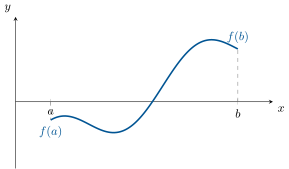
Theorem 13.10 (Intermediate value theorem)

Let $f$ be continuous on $\intcc{a}{b}$ with $f(a) \leq 0 \leq f(b)$ . Then $f(c) = 0$ for some $c \in \intcc{a}{b}$ . Consequently, a continuous function on an interval takes every value between any two of its values: $f(I)$ is an interval.

Proof. Dichotomy. Set $a_0 = a$ , $b_0 = b$ . Given $\intcc{a_n}{b_n}$ with $f(a_n) \leq 0 \leq f(b_n)$ , let $m$ be the midpoint: if $f(m) \leq 0$ keep $\intcc{m}{b_n}$ , otherwise keep $\intcc{a_n}{m}$ ; the sign conditions persist. The sequences $(a_n), (b_n)$ are adjacent ( $b_n - a_n = \frac{b-a}{2^n}$ ), with common limit $c$ (Theorem 11.11). By continuity and Theorem 11.7: $f(c) = \lim f(a_n) \leq 0$ and $f(c) = \lim f(b_n) \geq 0$ , so $f(c) = 0$ .

For the consequence: given values $f(u) < v < f(w)$ , apply the above to $x \mapsto f(x) - v$ on the segment with endpoints $u$ and $w$ ; thus $f(I)$ is convex, i.e. an interval (Proposition 10.19). ∎

A continuous function with f(a) < 0 < f(b) must cross the axis: the dichotomy proof of traps a crossing point between adjacent sequences. — A continuous function with $f(a) < 0 < f(b)$ must cross the axis: the dichotomy proof of Theorem 13.10 traps a crossing point between adjacent sequences.

Example 13.11 (One equation, the full protocol)

Solve $\eu^x = 3 - x$ over $\R$ : existence, uniqueness, location. Set $g(x) = \eu^x + x - 3$ , continuous. Location and existence: $g(0) = -2 < 0$ and $g(1) = \eu - 2 > 0$ , so the intermediate value theorem plants a solution in $\intoo{0}{1}$ . Uniqueness: $g$ is a sum of the strictly increasing $\eu^x$ and $x - 3$ , hence strictly increasing on $\R$ ; a strictly monotone function takes each value at most once, so the solution is unique on all of $\R$ (not just in the interval probed). The protocol — rearrange to $g = 0$ , sign change for existence, monotonicity for uniqueness — settles most “how many solutions” questions in three lines, and Chapter 14’s variation tables extend it to non-monotone $g$ by cutting $\R$ into monotone branches.

Example 13.12 (Dichotomy as an algorithm)

The proof of Theorem 13.10 computes. Take $f(x) = x^3 + x - 1$ : $f(0) = -1 < 0 < 1 = f(1)$ , so a root lies in $\intoo{0}{1}$ . Halving:

f(0.5) = -0.375 < 0, \qquad f(0.75) = 0.171875 > 0, \qquad f(0.625) = -0.130859375 < 0 ,

so the root is successively trapped in $\intoo{0.5}{1}$ , then $\intoo{0.5}{0.75}$ , then $\intoo{0.625}{0.75}$ (true value: $c \approx 0.6823$ ). After $n$ steps the error is at most $\frac{b - a}{2^n}$ : ten steps give three decimals, twenty give six. The closing insight: the intermediate value theorem is not only an existence statement — its dichotomy proof is a guaranteed, if slow, root-finding algorithm, against which the fast but local Newton method of Chapter 14 should be measured.

Theorem 13.13 (Extreme value theorem)

A continuous function on a segment $\intcc{a}{b}$ is bounded and attains its bounds: there are $c, d \in \intcc{a}{b}$ with

f(c) = \inf_{\intcc{a}{b}} f, \qquad f(d) = \sup_{\intcc{a}{b}} f .

Combined with Theorem 13.10: the continuous image of a segment is a segment $\intcc{f(c)}{f(d)}$ .

Proof. Bounded above: otherwise pick $u_n$ with $f(u_n) \geq n$ . By compactness of the segment (Theorem 12.19), a subsequence $u_{\varphi(n)} \to x \in \intcc{a}{b}$ ; continuity gives $f(u_{\varphi(n)}) \to f(x)$ , but $f(u_{\varphi(n)}) \geq \varphi(n) \to +\infty$ : contradiction.

Sup attained: let $M = \sup f$ and choose $v_n$ with $f(v_n) > M - \frac{1}{n+1}$ (Proposition 10.4). Extract $v_{\varphi(n)} \to d \in \intcc{a}{b}$ : then $f(d) = \lim f(v_{\varphi(n)}) = M$ by the squeeze. The infimum is handled by $-f$ . ∎

Example 13.14 (Positive minimum on a segment)

Let $f$ be continuous on $\intcc{0}{1}$ with $f(x) > 0$ for every $x$ . Then $\inf f > 0$ : by the extreme value theorem the infimum is a value $f(c)$ , and $f(c) > 0$ by hypothesis. So a continuous positive function on a segment is bounded away from $0$ — a two-line argument used a dozen times in the coming chapters (denominators under control, step-function framings, error bounds). On a non-compact interval this fails spectacularly: $f(x) = x$ on $\intoc{0}{1}$ is continuous and positive with $\inf f = 0$ , not attained. The closing insight: “positive” upgrades to “uniformly positive” exactly when the domain is compact; every hypothesis of the extreme value theorem is load-bearing.

Remark 13.15 (Common pitfalls around the three theorems)

(i) Continuous images: only segments are robust. The continuous image of an open interval need not be open ( $x \mapsto x^2$ maps $\intoo{-1}{1}$ onto $\intco{0}{1}$ ), the image of a closed set need not be closed ( $\arctan$ maps the closed $\R$ onto the open $\intoo{-\frac\pi2}{\frac\pi2}$ ); but the image of a segment is a segment (Theorem 13.13). (ii) The intermediate value theorem needs an interval: the function $x \mapsto \frac1x$ , continuous on $\intco{-1}{0} \cup \intoc{0}{1}$ , takes the values $-1$ and $1$ yet never vanishes — its domain is two disjoint pieces, and the value $0$ falls into the gap; always name the interval on which the theorem is applied. (iii) Uniform continuity is a property of the pair (function, set): $x^2$ is uniformly continuous on every segment yet not on $\R$ (Example 13.20) — the words “uniformly continuous” without a domain are meaningless. (iv) Continuity of the inverse is not formal: it holds on intervals via monotonicity (Theorem 13.16), but a continuous bijection between unions of intervals can have a discontinuous inverse — the remark after that theorem is there because students quote it without the interval hypothesis.

13.3 Monotone functions and inverse functions

Theorem 13.16 (Monotone bijection theorem)

Let $f$ be continuous and strictly monotonic on an interval $I$ . Then

$f$ is a bijection from $I$ onto the interval $J = f(I)$ ;
the inverse $f^{-1} \colon J \to I$ is strictly monotonic (in the same direction) and continuous.

Proof. Say $f$ is strictly increasing. (1) Injectivity is immediate from strict monotonicity; surjectivity onto $f(I)$ is trivial, and $f(I)$ is an interval by Theorem 13.10.

(2) $f^{-1}$ is strictly increasing: if $y < y'$ in $J$ but $f^{-1}(y) \geq f^{-1}(y')$ , applying the increasing $f$ gives $y \geq y'$ , absurd. Continuity of $f^{-1}$ at $y_0 = f(x_0) \in J$ : let $\varepsilon > 0$ . Suppose first $x_0$ interior to $I$ , and shrink $\varepsilon$ so that $x_0 \pm \varepsilon \in I$ : their images satisfy $f(x_0 - \varepsilon) < y_0 < f(x_0 + \varepsilon)$ . Take $\delta = \min\bigl(y_0 - f(x_0 - \varepsilon),\, f(x_0 + \varepsilon) - y_0\bigr) > 0$ : for $\abs{y - y_0} \leq \delta$ , monotonicity of $f^{-1}$ squeezes $f^{-1}(y)$ between $x_0 - \varepsilon$ and $x_0 + \varepsilon$ . If $x_0$ is, say, the left endpoint of $I$ , only $x_0 + \varepsilon$ is available: then $y_0 = \min J$ (monotonicity), every $y \in J$ with $y - y_0 \leq f(x_0 + \varepsilon) - y_0$ satisfies $x_0 \leq f^{-1}(y) \leq x_0 + \varepsilon$ , and the one-sided estimate is exactly continuity at an endpoint; the right endpoint is symmetric. (Note: continuity of $f^{-1}$ was not deduced from that of $f$ by symmetry — it is monotonicity on an interval that does the work.) ∎

Remark 13.17

This theorem is what Definition 4.9 and Proposition 4.21 silently used: $\arcsin$ , $\arccos$ , $\arctan$ , $\operatorname{arsinh}$ , … are continuous. A complement (Exercise 13.10): a continuous injective function on an interval is automatically strictly monotonic, so the monotonicity hypothesis costs nothing.

Example 13.18 (Roots of all orders)

For $n \in \N^*$ , the function $f(x) = x^n$ is continuous and strictly increasing on $\intco{0}{+\infty}$ , with $f(0) = 0$ and $f(x) \to +\infty$ : its image is $\intco{0}{+\infty}$ (Theorem 13.10 for the interval structure). The monotone bijection theorem then delivers, in one stroke, a strictly increasing continuous inverse

x \mapsto x^{1/n} \colon \intco{0}{+\infty} \to \intco{0}{+\infty} :

existence, uniqueness and continuity of $n$ -th roots, with no computation. Compare with Exercise 10.12, which built $\sqrt y$ by hand from the supremum: one chapter of theory has compressed that page of work into two lines, and the same two lines legitimized $\arcsin$ , $\arctan$ and $\operatorname{arsinh}$ before them. The closing insight: a good theorem is stored labor.

13.4 Uniform continuity

Definition 13.19

$f \colon I \to \R$ is uniformly continuous when

\forall \varepsilon > 0,\ \exists \delta > 0,\ \forall x, y \in I, \qquad \abs{x - y} \leq \delta \implies \abs{f(x) - f(y)} \leq \varepsilon .

The point: $\delta$ depends only on $\varepsilon$ , not on the location in $I$ . Uniform continuity implies continuity; a Lipschitz function ( $\abs{f(x) - f(y)} \leq k \abs{x - y}$ ) is uniformly continuous ( $\delta = \varepsilon/k$ ).

Example 13.20

$x \mapsto x^2$ is continuous on $\R$ but not uniformly continuous: $\abs{(n + \frac 1n)^2 - n^2} = 2 + \frac{1}{n^2} \geq 2$ although the arguments are at distance $\frac 1n \to 0$ . On any bounded interval it is Lipschitz, hence uniformly continuous — consistent with Heine’s theorem below.

Example 13.21 (Uniform moduli, explicitly)

On a segment, Heine guarantees a uniform $\delta$ ; often one can also compute it. For $f(x) = x^2$ on $\intcc{0}{10}$ :

\abs{x^2 - y^2} = \abs{x + y}\,\abs{x - y} \leq 20\,\abs{x - y},

so $\delta = \frac{\varepsilon}{20}$ works uniformly (a Lipschitz modulus, linear in $\varepsilon$ ). For $\sqrt x$ on $\intcc{0}{1}$ : $\abs{\sqrt x - \sqrt y} \leq \sqrt{\abs{x - y}}$ (Exercise 13.9), so $\delta = \varepsilon^2$ works — uniform but not linear: near $0$ the square root is steep, and the price appears in the exponent of $\varepsilon$ , not in a failure of uniformity. The closing insight: uniform continuity is a spectrum, not a yes/no — the function $\delta(\varepsilon)$ , called the modulus, measures how expensive the uniformity is, and Lipschitz is simply its best grade.

Theorem 13.22 (Heine)

A continuous function on a segment $\intcc{a}{b}$ is uniformly continuous.

Proof. By contradiction: suppose some $\varepsilon_0 > 0$ defeats every $\delta$ . With $\delta = \frac{1}{n+1}$ , pick $x_n, y_n \in \intcc{a}{b}$ with $\abs{x_n - y_n} \leq \frac{1}{n+1}$ and $\abs{f(x_n) - f(y_n)} > \varepsilon_0$ . Compactness (Theorem 12.19) extracts $x_{\varphi(n)} \to c \in \intcc{a}{b}$ ; then $y_{\varphi(n)} \to c$ too (squeeze on $\abs{x - y}$ ). Continuity at $c$ gives $f(x_{\varphi(n)}) \to f(c)$ and $f(y_{\varphi(n)}) \to f(c)$ , so $\abs{f(x_{\varphi(n)}) - f(y_{\varphi(n)})} \to 0 < \varepsilon_0$ : contradiction. ∎

Example 13.23 (Bounded, continuous, yet not uniformly so)

The function $f(x) = \sin(x^2)$ is continuous and bounded on $\R$ , but not uniformly continuous. Take

x_n = \sqrt{2\pi n}, \qquad y_n = \sqrt{2\pi n + \tfrac\pi2}: \qquad y_n - x_n = \frac{\pi/2}{\sqrt{2\pi n + \frac\pi2} + \sqrt{2\pi n}} \longrightarrow 0 ,

yet $f(y_n) - f(x_n) = \sin\bigl(2\pi n + \frac\pi2\bigr) - \sin(2\pi n) = 1 - 0 = 1$ for every $n$ : no single $\delta$ can serve $\varepsilon = \frac12$ everywhere. Geometrically, the oscillations of $\sin(x^2)$ accelerate: the graph completes a full wave over shorter and shorter windows, so the horizontal scale a given $\varepsilon$ requires shrinks to zero as $x$ grows. The closing insight: boundedness does not buy uniformity (this example), and unboundedness does not preclude it ( $\sqrt x$ , Exercise 13.9); what decides is the modulus of oscillation, and Heine’s theorem says compact domains discipline it automatically.

Example 13.24 (The calculator experiment, explained)

Type any number into a calculator and press $\cos$ repeatedly: the display locks onto $0.7390851\dots$ Why? After one press the value lies in $\intcc{-1}{1}$ , after two in $\intcc{\cos 1}{1} \subseteq \intcc{0.54}{1}$ , a stable interval for $\cos$ . On it, $\abs{\cos a - \cos b} \leq \sin(1)\,\abs{a - b}$ with $\sin 1 = 0.841\dots < 1$ (the product-to-sum bound of Problem 11.1, or the mean value inequality of Chapter 14): the iteration contracts, so by the error-control step of Method 11.23,

\abs{u_n - c} \leq (0.842)^{\,n-2}\,\abs{u_2 - c} \longrightarrow 0 ,

where $c$ is the unique fixed point $\cos c = c$ (Exercise 13.6). About $40$ presses buy three decimals ( $0.842^{40} \approx 10^{-3}$ ) — a geometric rate, milder than dichotomy’s $2^{-n}$ per step, but each press costs one keystroke while each dichotomy step costs a full sign evaluation. The closing insight: the fixed-point picture of Chapter 11 and the existence theorems of this chapter are two halves of one story — IVT finds $c$ , contraction reaches it.

Remark 13.25 (Where these theorems work next)

The three pillars of this chapter each power a later one. The intermediate value theorem feeds every existence-of-solutions argument and the monotone bijection theorem; the extreme value theorem turns optimization problems into theorems (Rolle and the mean value theorem in Chapter 14 start exactly there); Heine’s theorem is the reason continuous functions on segments can be integrated in Chapter 15 — the uniform $\delta$ is what makes Riemann sums converge. In the Year 2 volume the same trio reappears in normed vector spaces, with compactness doing the work that segments do here.

Remark 13.26 (Perspectives inside this volume)

Continuity is about to be outranked but never retired. Chapter 14 strengthens it to differentiability and returns the favor (differentiable implies continuous); Chapter 15 rests on it twice, through Heine for the construction and through the fundamental theorem, whose central object $x \mapsto \int_a^x f$ upgrades a merely continuous $f$ to a $C^1$ primitive. In Chapter 25, continuity in two variables holds a trap worth previewing: the function $\frac{xy}{x^2 + y^2}$ (extended by $0$ ) is continuous in $x$ for each fixed $y$ and in $y$ for each fixed $x$ , yet not continuous at the origin — along the diagonal $x = y$ it is constantly $\frac12$ . Separate continuity is strictly weaker than continuity: the sequential characterization survives the move to $\R^2$ , but sequences must be allowed to approach from every direction, not only along the axes.

13.5 Exercises

Exercise 13.1 ★

Using the sequential characterization, prove that $x \mapsto \sin\frac 1x$ has no limit at $0^+$ (exhibit two sequences). Does $x \mapsto x \sin\frac 1x$ have one?

Solution

Solution of Exercise 13.1.

Take $u_n = \frac{1}{2\pi n + \pi/2}$ and $v_n = \frac{1}{2\pi n}$ : both tend to $0^+$ , yet $\sin\frac{1}{u_n} = 1$ and $\sin\frac{1}{v_n} = 0$ . Two sequences, two different limits of images: by Theorem 13.3, no limit at $0^+$ .

$x \sin\frac1x$ : squeezed by $\abs{x\sin\frac1x} \leq \abs x \to 0$ , so the limit at $0$ exists and equals $0$ .

Exercise 13.2 ★

Study the continuity on $\R$ of $f(x) = \lfloor x \rfloor$ and of $g(x) = x - \lfloor x \rfloor$ , and of $h(x) = \lfloor x \rfloor + (x - \lfloor x\rfloor)^2$ .

Solution

Solution of Exercise 13.2.

$f = \lfloor\cdot\rfloor$ is continuous on $\R \setminus \Z$ (locally constant) and discontinuous at each $n \in \Z$ : left limit $n - 1$ , value $n$ .

$g(x) = x - \lfloor x\rfloor$ : same discontinuity points (the identity is continuous, so $g$ inherits the jumps of $f$ ); at $n \in \Z$ , left limit $1 \neq 0 = g(n)$ .

$h(x) = \lfloor x\rfloor + (x - \lfloor x\rfloor)^2$ : on $\intco{n}{n + 1}$ , $h(x) = n + (x - n)^2$ , continuous there; at $x = n$ , the left limit is $(n-1) + 1 = n = h(n)$ : the jumps cancel. $h$ is continuous on $\R$ (and strictly increasing).

Exercise 13.3 ★

Prove that the equation $x^5 - 3x + 1 = 0$ has at least three real solutions (evaluate at well-chosen points and apply Theorem 13.10 on three disjoint segments).

Solution

Solution of Exercise 13.3.

$P(x) = x^5 - 3x + 1$ : $P(-2) = -32 + 6 + 1 = -25 < 0$ ; $P(0) = 1 > 0$ ; $P(1) = -1 < 0$ ; $P(2) = 27 > 0$ . Three sign changes on the disjoint segments $\intcc{-2}{0}$ , $\intcc{0}{1}$ , $\intcc{1}{2}$ : by Theorem 13.10, at least three roots. (Being of degree $5$ , $P$ has at most five; a variation study would show exactly three.)

Exercise 13.4 ★

Prove that every polynomial of odd degree has a real root.

Solution

Solution of Exercise 13.4.

Let $P = a_{2m+1}X^{2m+1} + \dots$ with $a_{2m+1} > 0$ (else replace $P$ by $-P$ ). Factoring the dominant term, $P(x) = a_{2m+1} x^{2m+1}\bigl(1 + o(1)\bigr)$ as $x \to \pm\infty$ : so $P(x) \to +\infty$ at $+\infty$ and $-\infty$ at $-\infty$ . Pick $a$ with $P(a) < 0$ and $b$ with $P(b) > 0$ : the intermediate value theorem on $\intcc{a}{b}$ provides a root.

Exercise 13.5 ★★

(Fixed point) Let $f \colon \intcc{0}{1} \to \intcc{0}{1}$ be continuous. Prove that $f$ has a fixed point: $f(c) = c$ for some $c$ . Illustrate that neither continuity nor the segment can be dropped.

Solution

Solution of Exercise 13.5.

Let $g(x) = f(x) - x$ , continuous on $\intcc{0}{1}$ . Since $f$ maps into $\intcc{0}{1}$ : $g(0) = f(0) \geq 0$ and $g(1) = f(1) - 1 \leq 0$ . By Theorem 13.10, $g(c) = 0$ for some $c$ : a fixed point.

Necessity of the hypotheses: on $\intcc{0}{1}$ , the discontinuous map $f(x) = 1$ for $x \leq \frac12$ , $f(x) = 0$ for $x > \frac12$ has no fixed point; on the interval $\intoo{0}{1}$ (not a segment), $f(x) = \frac x2$ is continuous into $\intoo{0}{1}$ with no fixed point (the candidate $0$ is missing); on $\R$ , $f(x) = x + 1$ .

Exercise 13.6 ★★

Prove that the equation $\cos x = x$ has exactly one real solution, and that it lies in $\intoo{0}{1}$ .

Solution

Solution of Exercise 13.6.

$g(x) = \cos x - x$ is continuous, $g(0) = 1 > 0$ , $g(1) = \cos 1 - 1 < 0$ : a solution exists in $\intoo{0}{1}$ (Theorem 13.10). Uniqueness: $g$ is strictly decreasing on $\R$ — for $x \leq 0$ , $g(x) \geq 1 - x > 0$ has no zero anyway; and $g'(x) = -\sin x - 1 \leq 0$ with equality only at isolated points ( $x \equiv -\frac\pi2 \bmod 2\pi$ ), so $g$ is strictly decreasing (Chapter 14; alternatively: on $\intcc{0}{1}$ , $\cos$ is strictly decreasing and $-x$ too, so $g$ is). A strictly monotone function vanishes at most once.

Exercise 13.7 ★★

Let $f \colon \R \to \R$ be continuous with $f(x) \to +\infty$ as $x \to \pm\infty$ . Prove that $f$ attains a global minimum on $\R$ . (Reduce to a segment containing a sublevel set.)

Solution

Solution of Exercise 13.7.

Fix $M = f(0) + 1$ . There is $A > 0$ with $f(x) \geq M$ for $\abs x \geq A$ (definition of the two infinite limits; take the larger threshold). On the segment $\intcc{-A}{A}$ , the extreme value theorem (Theorem 13.13) provides $c$ with $f(c) = \inf_{\intcc{-A}{A}} f \leq f(0)$ . For $\abs x \geq A$ : $f(x) \geq M > f(0) \geq f(c)$ . So $f(c)$ is the global minimum.

Exercise 13.8 ★★

Let $f \colon \R \to \R$ be continuous and periodic (of period $T > 0$ ). Prove that $f$ is bounded and attains its bounds, and that there exists $c$ with $f(c + \frac T2) = f(c)$ . (For the second point, study $g(x) = f(x + \frac T2) - f(x)$ over one period.)

Solution

Solution of Exercise 13.8.

On the segment $\intcc{0}{T}$ , $f$ is bounded and attains its bounds (Theorem 13.13); by periodicity, these are the bounds on all of $\R$ , still attained.

Let $g(x) = f(x + \frac T2) - f(x)$ , continuous. Then

g(0) + g\bigl(\tfrac T2\bigr) = \bigl(f(\tfrac T2) - f(0)\bigr) + \bigl(f(T) - f(\tfrac T2)\bigr) = f(T) - f(0) = 0 :

$g(0)$ and $g(\frac T2)$ have opposite signs (or one vanishes), so the intermediate value theorem on $\intcc{0}{T/2}$ gives $c$ with $g(c) = 0$ , i.e. $f(c + \frac T2) = f(c)$ .

Exercise 13.9 ★★

Prove that $x \mapsto \sqrt x$ is uniformly continuous on $\intco{0}{+\infty}$ , although it is not Lipschitz near $0$ . (Prove and use $\abs{\sqrt x - \sqrt y} \leq \sqrt{\abs{x - y}}$ .)

Solution

Solution of Exercise 13.9.

First the inequality: for $0 \leq y \leq x$ ,

\bigl(\sqrt y + \sqrt{x - y}\bigr)^2 = x + 2\sqrt{y(x-y)} \geq x,

so $\sqrt x \leq \sqrt y + \sqrt{x - y}$ , i.e. $\sqrt x - \sqrt y \leq \sqrt{x - y}$ . Hence $\abs{\sqrt x - \sqrt y} \leq \sqrt{\abs{x - y}}$ for all $x, y \geq 0$ .

Uniform continuity: given $\varepsilon > 0$ , take $\delta = \varepsilon^2$ ; then $\abs{x - y} \leq \delta$ implies $\abs{\sqrt x - \sqrt y} \leq \sqrt\delta = \varepsilon$ .

Not Lipschitz near $0$ : $\frac{\sqrt x - \sqrt 0}{x - 0} = \frac{1}{\sqrt x} \to +\infty$ as $x \to 0^+$ , so no constant $k$ can dominate all difference quotients.

Exercise 13.10 ★★★

Let $f$ be continuous and injective on an interval $I$ . Prove that $f$ is strictly monotonic. Hint: if not, there are $a < b < c$ with, say, $f(b) > f(a)$ and $f(b) > f(c)$ ; apply the intermediate value theorem to a value between $\max(f(a), f(c))$ and $f(b)$ on both sides of $b$ .

Solution

Solution of Exercise 13.10.

Suppose $f$ is injective, continuous, and not strictly monotonic. Then there are $a < b < c$ in $I$ with $f(b)$ not between $f(a)$ and $f(c)$ — indeed, if for all triples the middle value were between the outer ones, $f$ would be monotonic (compare any two pairs; a short case check). Say $f(b) > \max(f(a), f(c))$ (the other case is symmetric, replace $f$ by $-f$ ). Choose $v$ with $\max(f(a), f(c)) < v < f(b)$ . By the intermediate value theorem applied on $\intcc{a}{b}$ and on $\intcc{b}{c}$ , there are $u_1 \in \intoo{a}{b}$ and $u_2 \in \intoo{b}{c}$ with $f(u_1) = v = f(u_2)$ : two distinct points with equal images, contradicting injectivity.

Exercise 13.11 ★★★

(Cauchy’s functional equation, continuous case) Let $f \colon \R \to \R$ be continuous with $f(x + y) = f(x) + f(y)$ for all $x, y$ . Prove that $f(x) = f(1)\,x$ for all $x$ : first on $\N$ , $\Z$ , $\Q$ (by additivity alone), then on $\R$ by continuity and density (Theorem 10.14).

Solution

Solution of Exercise 13.11.

$f(0) = f(0+0) = 2f(0)$ gives $f(0) = 0$ ; $f(-x) = -f(x)$ from $0 = f(x - x)$ . Set $\alpha = f(1)$ . Induction: $f(n) = n\alpha$ for $n \in \N$ , then for $n \in \Z$ by oddness. For $q \in \N^*$ : $q\,f(\frac pq) = f(p) = p\alpha$ (add $\frac pq$ to itself $q$ times), so $f(\frac pq) = \alpha\frac pq$ : $f = \alpha\, \mathrm{id}$ on $\Q$ .

Let now $x \in \R$ and $(r_n)$ a sequence of rationals with $r_n \to x$ (density, Theorem 10.14, applied in nested intervals; or $r_n = \frac{\lfloor nx\rfloor}{n}$ ). Continuity: $f(x) = \lim f(r_n) = \lim \alpha r_n = \alpha x$ .

Exercise 13.12 ★★★

Let $f \colon \intco{0}{+\infty} \to \R$ be continuous with $f(x) \to \ell \in \R$ as $x \to +\infty$ . Prove that $f$ is uniformly continuous on $\intco{0}{+\infty}$ . (Cut at a large $A$ : Heine on $\intcc{0}{A+1}$ , the limit beyond $A$ ; make the two regimes overlap.)

Solution

Solution of Exercise 13.12.

Let $\varepsilon > 0$ . By the limit at $+\infty$ , there is $A$ with $\abs{f(x) - \ell} \leq \frac\varepsilon2$ for $x \geq A$ ; hence for $x, y \geq A$ : $\abs{f(x) - f(y)} \leq \varepsilon$ (no closeness needed).

On the segment $\intcc{0}{A + 1}$ , Heine’s theorem (Theorem 13.22) gives $\delta_0 > 0$ for this $\varepsilon$ ; set $\delta = \min(\delta_0, 1)$ .

Now take any $x, y \geq 0$ with $\abs{x - y} \leq \delta$ , say $x \leq y$ . If $y \leq A + 1$ : both lie in the segment, and the Heine $\delta_0$ applies. Otherwise $y > A + 1$ , and then $x \geq y - 1 > A$ : both lie in $\intco{A}{+\infty}$ , where the limit argument applies. In both cases $\abs{f(x) - f(y)} \leq \varepsilon$ : uniform continuity.

13.6 Problem: Cauchy’s functional equation and its sisters

Problem 13.1

Weekend problem — $f(x + y) = f(x) + f(y)$ : regularity forces linearity, and the portrait of the monsters

Which functions satisfy $f(x + y) = f(x) + f(y)$ for all real $x, y$ ? Cauchy raised the question in 1821; the answer is a paradigm. Exercise 13.11 shows that such an additive function is linear on $\Q$ and that full continuity forces $f(x) = cx$ . This problem sharpens the hypothesis dramatically — continuity at a single point, or monotonicity, or mere boundedness on one small interval, each suffices — then paints the portrait of a hypothetical nonlinear solution (its graph fills the plane), solves the sister equations characterizing $\eu^{cx}$ , $c\ln x$ , $x^c$ and $cx^2$ , and closes with Jensen’s equation and the theorem midpoint-convex $+$ continuous $\implies$ convex. Throughout, additive means: $f(x + y) = f(x) + f(y)$ for all $x, y \in \R$ .

Part I — $\Q$ -linearity, and one point of continuity.

Let $f$ be additive. From Exercise 13.11, $f(r) = f(1)\,r$ for rational $r$ . Prove the finer statement used below: for every $x \in \R$ and $r \in \Q$ , $f(rx) = r\,f(x)$ ( $f$ is $\Q$ -linear).
Suppose the additive $f$ is continuous at one single point $x_0$ . Show that $f$ is continuous everywhere (compute $f(x + h) - f(x)$ in terms of $f(x_0 + h) - f(x_0)$ ), hence $f(x) = f(1)\,x$ .
Show that an additive function is determined by its restriction to any dense subgroup: if two additive functions agree on $\Z + \sqrt2\,\Z$ and both are continuous, they are equal — while without continuity, prescribing $f(1) = 0$ and $f(\sqrt 2) = 1$ is consistent with $\Q$ -linearity on the subgroup. Compute $f(m + n\sqrt2)$ for this prescription.
Let $f$ be additive and bounded above by $M$ on some interval $\intcc{a}{b}$ with $a < b$ . Show that $f$ is bounded above on $\intcc{0}{\ell}$ , $\ell = b - a$ (translate by $a$ ).

Part II — The regularity ladder.

Continuing question 4: using $f(\ell - t) + f(t) = f(\ell)$ , show that $f$ is also bounded below on $\intcc{0}{\ell}$ : $\abs f \leq C$ there.
Show that $\abs{f(t)} \leq \frac{C}{n}$ for $t \in \intcc{0}{\ell/n}$ , and deduce that $f$ is continuous at $0$ (oddness handles the left side), hence everywhere (question 2): an additive function bounded on one interval is linear.
Deduce the monotone case: an additive function nondecreasing on some $\intcc{a}{b}$ ( $a < b$ ) is $f(x) = cx$ with $c \geq 0$ .
Assemble the regularity ladder: for an additive $f$ , the following are equivalent — (a) $f(x) = cx$ ; (b) $f$ continuous; (c) $f$ continuous at one point; (d) $f$ monotone on some nondegenerate interval; (e) $f$ bounded on some nondegenerate interval. Arrange the implications so that each is either trivial or already proved.
Verify that questions 4–6 consumed only a bound above: an additive function bounded above on one nondegenerate interval is already linear. Deduce the mirror statement for a bound below, and record the strongest form of the ladder’s rung (e) thus obtained.

Part III — Portrait of a monster. Suppose now $f$ is additive but not linear.

Show there are nonzero reals $u, v$ with $\dfrac{f(u)}{u} \neq \dfrac{f(v)}{v}$ , and that the vectors $(u, f(u))$ and $(v, f(v))$ span the plane (their determinant $u f(v) - v f(u)$ is nonzero).
Show that the graph of $f$ contains all points

$r\,(u, f(u)) + s\,(v, f(v)), \qquad r, s \in \Q ,$

and deduce that the graph is dense in $\R^2$ : for every point $(x_0, y_0)$ of the plane and every $\varepsilon > 0$ , some $(x, f(x))$ is within $\varepsilon$ of it (solve the $2\times2$ real system, then approximate the real coefficients by rationals).
Deduce from question 11 the full portrait: a nonlinear additive function is unbounded on every nondegenerate interval, discontinuous at every point, monotone on no interval, and its image of any interval is dense in $\R$ . Reconcile with question 8.
Monsters exist — on a dense subgroup, constructively: on $G = \Z + \sqrt2\,\Z$ define $f(m + n\sqrt2) = n$ . Show $f$ is well defined and additive on $G$ , and that $f$ is unbounded on $G \cap \intoo{0}{\varepsilon}$ for every $\varepsilon > 0$ (for fixed $N$ , only finitely many $g = m + n\sqrt2 \in \intoo{0}{1}$ have $\abs n \leq N$ ; yet $G \cap \intoo{0}{\varepsilon}$ is infinite). Explain in one paragraph why extending such an $f$ to all of $\R$ requires a basis of $\R$ as a $\Q$ -vector space (a Hamel basis), whose existence is an axiom-of-choice matter beyond this volume.

Part IV — The sister equations. All functions here are continuous.

Let $f \colon \R \to \R$ be continuous, not identically $0$ , with $f(x + y) = f(x)f(y)$ . Show $f(x) = f\bigl(\frac x2\bigr)^2 \geq 0$ , then $f > 0$ everywhere, then $f(x) = \eu^{cx}$ for some $c$ : the exponentials are exactly the continuous morphisms from $(\R, +)$ to $(\R^*, \times)$ .
Let $f \colon \intoo{0}{+\infty} \to \R$ be continuous with $f(xy) = f(x) + f(y)$ . Show $f(x) = c\ln x$ (transport by $\exp$ ).
Let $f \colon \intoo{0}{+\infty} \to \intoo{0}{+\infty}$ be continuous with $f(xy) = f(x)f(y)$ . Show $f(x) = x^c$ .
Find all continuous $f \colon \R \to \R$ with

$f(x + y) = f(x) + f(y) + f(x)f(y) .$

(Study $h = 1 + f$ ; treat the degenerate case separately.)
(Parallelogram) Find all continuous $f \colon \R \to \R$ with $f(x + y) + f(x - y) = 2f(x) + 2f(y)$ : show $f$ is even, $f(0) = 0$ , $f(nx) = n^2 f(x)$ by induction, then $f(x) = f(1)\,x^2$ . (This equation is the fingerprint of quadratic forms — the parallelogram law that detects, in the Year 2 volume, which norms come from an inner product.)

Part V — Jensen and midpoint convexity.

(Jensen’s equation) Let $f \colon \R \to \R$ be continuous with $f\bigl(\frac{x+y}{2}\bigr) = \frac{f(x) + f(y)}{2}$ . Show that $g = f - f(0)$ satisfies $g\bigl(\frac x2\bigr) = \frac{g(x)}{2}$ , deduce that $g$ is additive, and conclude $f(x) = cx + d$ .
Suppose now only the inequality: $f$ continuous with

$f\Bigl(\frac{x + y}{2}\Bigr) \leq \frac{f(x) + f(y)}{2} \qquad (x, y \in \R).$

Prove by induction on $n$ that for all dyadic weights $\lambda = \frac{k}{2^n} \in \intcc{0}{1}$ :

$f\bigl(\lambda x + (1 - \lambda)y\bigr) \leq \lambda f(x) + (1 - \lambda) f(y) .$
Extend by continuity and density of the dyadics (Exercise 10.8) to every $\lambda \in \intcc{0}{1}$ : a continuous midpoint-convex function satisfies the full convexity inequality (the notion studied systematically in Chapter 14).
Show continuity cannot be dropped: a nonlinear additive $f$ satisfies the midpoint equality of question 19 yet no convexity inequality on any interval (question 12). Moral: midpoint convexity is a countable-stage property (dyadics), convexity a continuum one; continuity is the bridge — exactly as in Parts I–II.

Part VI — Last variations and synthesis.

Find all continuous $f \colon \R \to \R$ with $f(x + y) = f(x) + f(y) + xy$ (subtract the particular solution $\frac{x^2}{2}$ ).
Prove: if $f \colon \R \to \R$ is continuous and additive merely on a dense subgroup $G$ (i.e. $f(g + g') = f(g) + f(g')$ for $g, g' \in G$ ), then $f$ is additive on $\R$ . More generally, two continuous functions that agree on a dense subset of $\R$ are equal.
Synthesis, one sentence each: (i) state the regularity ladder of question 8 from memory; (ii) explain why “graph dense in the plane” is the right mental image for the failure of regularity; (iii) list the five classical functions characterized in Part IV–V and the single method that caught them all; (iv) name the two places where density of $\Q$ (or of the dyadics) in $\R$ carried the argument, and the place where it could not (question 13).

Solution

Solution of Problem 13.1.

1. For $n \in \N$ : $f(nx) = n f(x)$ by induction ( $f((n+1)x) = f(nx) + f(x)$ ). Also $f(0) = 2f(0)$ gives $f(0) = 0$ , and $0 = f(x - x) = f(x) + f(-x)$ gives oddness, so $f(nx) = nf(x)$ for $n \in \Z$ . For $r = \frac pq$ : $q\,f\bigl(\tfrac pq x\bigr) = f(px) = p\,f(x)$ , so $f(rx) = r f(x)$ : $f$ is $\Q$ -linear.

2. Additivity gives, for all $x$ and $h$ :

f(x + h) - f(x) = f(h) = f(x_0 + h) - f(x_0) .

As $h \to 0$ , the right side tends to $0$ by continuity at $x_0$ ; hence $f(x + h) \to f(x)$ : continuity at every $x$ . Then Exercise 13.11 yields $f(x) = f(1)\,x$ .

3. Two continuous additive functions are of the form $cx$ and $c'x$ (question 2); if they agree on the dense subgroup $\Z + \sqrt2\,\Z$ (Exercise 10.9), then $c\,g = c'g$ for some $g \neq 0$ in it: $c = c'$ , the functions are equal. Without continuity: $\Q$ -linearity only ties values at $\Q$ -combinations, and $1, \sqrt2$ are $\Q$ -independent ( $\sqrt2 \notin \Q$ ), so $f(1) = 0$ , $f(\sqrt2) = 1$ is consistent and forces, on the subgroup,

f(m + n\sqrt2) = m\,f(1) + n\,f(\sqrt2) = n .

4. For $t \in \intcc{0}{\ell}$ : $a + t \in \intcc{a}{b}$ , so $f(t) = f(a + t) - f(a) \leq M - f(a) =: M'$ .

5. For $t \in \intcc{0}{\ell}$ , also $\ell - t \in \intcc{0}{\ell}$ , and additivity gives $f(t) = f(\ell) - f(\ell - t) \geq f(\ell) - M'$ . Hence $\abs{f} \leq C$ on $\intcc{0}{\ell}$ with $C = \max\bigl(\abs{M'}, \abs{f(\ell) - M'}\bigr)$ .

6. For $t \in \intcc{0}{\ell/n}$ : $nt \in \intcc{0}{\ell}$ and $f(t) = \frac{f(nt)}{n}$ (question 1), so $\abs{f(t)} \leq \frac Cn$ . Given $\varepsilon > 0$ , choose $n > \frac C\varepsilon$ : for $0 \leq h \leq \frac\ell n$ , $\abs{f(h)} \leq \varepsilon$ , and for negative $h$ use $f(h) = -f(-h)$ . So $f(h) \to 0 = f(0)$ as $h \to 0$ : continuity at $0$ , hence everywhere (question 2), hence $f(x) = f(1)x$ .

7. If $f$ is nondecreasing on $\intcc{a}{b}$ , then $f(a) \leq f(x) \leq f(b)$ there: bounded, so linear by question 6, $f(x) = cx$ ; and $c(b - a) = f(b) - f(a) \geq 0$ forces $c \geq 0$ .

8. (a) $\Rightarrow$ (b) $\Rightarrow$ (c): trivial. (c) $\Rightarrow$ (a): question 2. (a) $\Rightarrow$ (d): a linear function is monotone everywhere. (d) $\Rightarrow$ (e): a monotone function on $\intcc{a}{b}$ is bounded there by its endpoint values. (e) $\Rightarrow$ (a): questions 4–6. The five statements are equivalent — the regularity ladder.

9. Question 4 used only the upper bound $M$ ; question 5 derived the lower bound from the upper one via the reflection $f(t) = f(\ell) - f(\ell - t)$ ; question 6 then ran on $\abs f \leq C$ . So: additive and bounded above on one nondegenerate interval already implies linear. For a bound below, apply this to $-f$ (additive, bounded above). Strongest rung (e): a one-sided bound on one interval suffices.

10. If $\frac{f(x)}{x}$ were one constant $c$ for all $x \neq 0$ , $f$ would be linear; so there are nonzero $u, v$ with $\frac{f(u)}u \neq \frac{f(v)}v$ , i.e. $u f(v) - v f(u) \neq 0$ : the determinant of the vectors $(u, f(u))$ , $(v, f(v))$ is nonzero, and they span $\R^2$ .

11. For $r, s \in \Q$ : $f(ru + sv) = r f(u) + s f(v)$ (question 1 twice plus additivity), so the graph contains

\bigl(ru + sv,\; r f(u) + s f(v)\bigr) = r\,(u, f(u)) + s\,(v, f(v)) .

Given $(x_0, y_0)$ and $\varepsilon > 0$ : the $2 \times 2$ system $a(u, f(u)) + b(v, f(v)) = (x_0, y_0)$ has a (unique) real solution $(a, b)$ since the determinant is nonzero. Pick rationals $r_n \to a$ , $s_n \to b$ : then $r_n(u, f(u)) + s_n(v, f(v)) \to (x_0, y_0)$ coordinatewise, and each of these points lies on the graph: the graph is dense in $\R^2$ .

12. Let $I$ be a nondegenerate interval, $x_0$ its midpoint, $M$ arbitrary: density provides a graph point within $\min\bigl(\frac{\abs I}{2}, 1\bigr)$ of $(x_0, M + 1)$ , i.e. $x \in I$ with $f(x) > M$ : unbounded on $I$ , hence (question 8) discontinuous at every point and monotone on no interval; and for any target $y_0$ , graph points near $(x_0, y_0)$ give $f(x)$ arbitrarily close to $y_0$ with $x \in I$ : $f(I)$ is dense in $\R$ . This is question 8 read backwards: since all rungs are equivalent, a nonlinear additive function must fail all of them, everywhere.

13. Well defined: $m + n\sqrt2 = m' + n'\sqrt2$ forces $(n - n')\sqrt2 = m' - m \in \Z$ , so $n = n'$ (else $\sqrt2 \in \Q$ ) and $m = m'$ . Additivity on $G$ is then clear coordinate by coordinate. Unboundedness near $0^+$ : fix $\varepsilon \in \intoo{0}{1}$ and $N \in \N$ . For each fixed $n$ with $\abs n \leq N$ , the condition $m + n\sqrt2 \in \intoo{0}{1}$ pins $m$ inside an interval of length $1$ : at most one integer $m$ per $n$ , so at most $2N + 1$ elements of $G \cap \intoo{0}{1}$ have $\abs{f} \leq N$ . But $G \cap \intoo{0}{\varepsilon}$ is infinite ( $G$ is dense, Exercise 10.9); hence it contains some $g$ with $\abs{f(g)} > N$ : $f$ is unbounded on every right neighborhood of $0$ . Extending $f$ to an additive function on $\R$ means choosing values coherently on a family of reals that is $\Q$ -linearly independent and spans $\R$ over $\Q$ — a Hamel basis; producing one requires the axiom of choice, and no explicit formula can do it: constructively we own the monster only on $G$ .

14. $f(x) = f(\frac x2 + \frac x2) = f(\frac x2)^2 \geq 0$ . If $f(x_0) = 0$ , then $f(x) = f(x - x_0)f(x_0) = 0$ for all $x$ : excluded. So $f > 0$ and $g = \ln \circ f$ is continuous (Proposition 13.8) with $g(x + y) = g(x) + g(y)$ : by Exercise 13.11, $g(x) = cx$ , so $f(x) = \eu^{cx}$ . Conversely each $\eu^{cx}$ works: the continuous morphisms $(\R, +) \to (\R^*, \times)$ are exactly the exponentials.

15. $g(u) = f(\eu^u)$ is continuous and $g(u + v) = f(\eu^u \eu^v) = g(u) + g(v)$ : $g(u) = cu$ , and every $x > 0$ writes $x = \eu^u$ with $u = \ln x$ : $f(x) = c\ln x$ .

16. $h = \ln \circ f$ is continuous on $\intoo{0}{+\infty}$ with $h(xy) = h(x) + h(y)$ : by question 15, $h(x) = c\ln x$ , so $f(x) = \eu^{c\ln x} = x^c$ .

17. $x = y = 0$ : $f(0) = 2f(0) + f(0)^2$ , so $f(0)(1 + f(0)) = 0$ . If $f(0) = -1$ : setting $y = 0$ , $f(x) = f(x) + f(0) + f(x)f(0) = -1$ for all $x$ : the constant $f \equiv -1$ (which indeed satisfies the equation). Otherwise $f(0) = 0$ ; $h = 1 + f$ is continuous, $h(0) = 1$ , and

h(x + y) = 1 + f(x) + f(y) + f(x)f(y) = h(x)\,h(y) :

by question 14, $h(x) = \eu^{cx}$ , i.e. $f(x) = \eu^{cx} - 1$ (the case $c = 0$ giving $f \equiv 0$ ). Complete list: $f \equiv -1$ and $f(x) = \eu^{cx} - 1$ , $c \in \R$ .

18. $x = y = 0$ : $2f(0) = 4f(0)$ , so $f(0) = 0$ . $x = 0$ : $f(y) + f(-y) = 2f(y)$ , so $f$ is even. $y = x$ : $f(2x) = 4f(x)$ . Induction using $(x, y) \to (nx, x)$ :

f((n{+}1)x) = 2f(nx) + 2f(x) - f((n{-}1)x) = (2n^2 + 2 - (n-1)^2) f(x) = (n+1)^2 f(x) .

Then $f(x) = f\bigl(q\cdot\frac xq\bigr) = q^2 f\bigl(\frac xq\bigr)$ gives $f\bigl(\frac pq x\bigr) = \frac{p^2}{q^2}f(x)$ : $f(r) = r^2 f(1)$ on $\Q$ (evenness handles signs). The two continuous functions $f$ and $x \mapsto f(1)x^2$ agree on the dense set $\Q$ , hence everywhere (question 24): $f(x) = f(1)\,x^2$ ; every $cx^2$ satisfies the equation.

19. $g = f - f(0)$ is continuous, $g(0) = 0$ , and satisfies Jensen’s equation (the constants cancel). Taking $y = 0$ : $g\bigl(\frac x2\bigr) = \frac{g(x)}{2}$ . Then for all $x, y$ :

\frac{g(x + y)}{2} = g\Bigl(\frac{x+y}{2}\Bigr) = \frac{g(x) + g(y)}{2} ,

so $g$ is additive and continuous: $g(x) = cx$ (question 2), and $f(x) = cx + d$ with $d = f(0)$ . All affine functions satisfy Jensen: the list is complete.

20. Induction on $n$ . For $n = 0$ : $\lambda \in \{0, 1\}$ , trivial. Assume the inequality for all weights $\frac{k}{2^n}$ . A weight $\lambda = \frac{k}{2^{n+1}}$ with $k$ even reduces to level $n$ ; for $k = 2j + 1$ , $\lambda$ is the midpoint of $\lambda_1 = \frac{j}{2^n}$ and $\lambda_2 = \frac{j+1}{2^n}$ . With $z_i = \lambda_i x + (1 - \lambda_i)y$ : $\lambda x + (1-\lambda)y = \frac{z_1 + z_2}{2}$ , so

f\bigl(\lambda x + (1{-}\lambda)y\bigr) \leq \frac{f(z_1) + f(z_2)}{2} \leq \frac{(\lambda_1 + \lambda_2)f(x) + (2 - \lambda_1 - \lambda_2)f(y)}{2} = \lambda f(x) + (1 - \lambda)f(y) .

21. Fix $x, y$ . The maps $\lambda \mapsto f(\lambda x + (1 - \lambda)y)$ and $\lambda \mapsto \lambda f(x) + (1 - \lambda)f(y)$ are continuous on $\intcc{0}{1}$ (composition and algebra, Proposition 13.8). The inequality holds on the dyadic weights, which are dense in $\intcc{0}{1}$ (Exercise 10.8); for arbitrary $\lambda$ take dyadics $\lambda_n \to \lambda$ and pass to the limit (Theorem 13.3 and Theorem 11.7): the convexity inequality holds for every $\lambda \in \intcc{0}{1}$ — midpoint convexity plus continuity equals convexity (the notion of Chapter 14).

22. A nonlinear additive $f$ satisfies $f\bigl(\frac{x+y}{2}\bigr) = \frac{f(x) + f(y)}{2}$ exactly (question 1 with $r = \frac12$ , then additivity): it is midpoint-convex, even midpoint-affine. If it satisfied the full convexity inequality on some interval $\intcc{x}{y}$ , then for $\lambda \in \intcc{0}{1}$ : $f(\lambda x + (1-\lambda)y) \leq \max(f(x), f(y))$ — bounded above on a nondegenerate interval, hence linear by question 9: contradiction. So continuity in question 21 is not a luxury: without it, midpoint convexity controls only the countable dyadic skeleton, and the continuum in between runs wild.

23. $p(x) = \frac{x^2}{2}$ satisfies $p(x+y) = p(x) + p(y) + xy$ . If $f$ is any continuous solution, $g = f - p$ is continuous and additive, so $g(x) = cx$ :

f(x) = \frac{x^2}{2} + cx , \qquad c \in \R ,

and each of these is a solution: the list is complete.

24. General principle: if $u, v$ are continuous and agree on a dense $D \subseteq \R$ , then for $x \in \R$ choose $d_n \in D$ with $d_n \to x$ (Proposition 12.11); $u(x) = \lim u(d_n) = \lim v(d_n) = v(x)$ . Now let $f$ be continuous and additive on the dense subgroup $G$ . Fix $x, y \in \R$ and take $g_n \to x$ , $g'_n \to y$ with $g_n, g'_n \in G$ ; then $g_n + g'_n \to x + y$ and, by sequential continuity at $x + y$ , $x$ and $y$ :

f(x + y) = \lim f(g_n + g'_n) = \lim\bigl(f(g_n) + f(g'_n)\bigr) = f(x) + f(y) :

$f$ is additive on all of $\R$ (hence linear, by question 2).

25. (i) For additive $f$ : linear $\iff$ continuous $\iff$ continuous at one point $\iff$ monotone on some interval $\iff$ bounded (even one-sidedly) on some interval. (ii) Density of the graph in the plane shows the failure is not a local defect but a global explosion: above every subinterval the values smear over all of $\R$ , so every regularity property fails everywhere at once. (iii) The catch: $cx$ , $\eu^{cx}$ , $c\ln x$ , $x^c$ , $cx^2$ , and $cx + d$ — six characterizations, one method: transport the equation to Cauchy’s, prove the $\Q$ -skeleton by induction, upgrade to $\R$ by density plus continuity. (iv) Density of $\Q$ (or the dyadics) carried the upgrades in Exercise 13.11 and in question 21; it carried nothing in question 13, because without continuity values do not propagate from a dense set to its closure — density transfers information only along continuity.