The Desk and the Firm · The firm
8Managing a Book through Drawdown
Two portfolio managers are both down eight per cent from their peak in March. One runs a strategy that has had a bad few months; the other’s edge died a year ago and nobody has noticed. On the day each first reaches the eight per cent, the best statistical reading of their P&L gives the first a 24% chance of having broken and the second 39%: the numbers barely differ. To tell a strategy whose Sharpe ratio has fallen from 1 to 0 from one that is merely unlucky, at a false-alarm rate of one in ten years, takes on average more than fifteen years of data. The head of desk must decide in March.
8.1 What a drawdown says about a Sharpe ratio
A drawdown (One Quant Book 2, chapter 29) is the fall of cumulative P&L from its running peak; its maximum over a period and its duration are Book 7’s measures (chapter 22). What matters for management is how large a drawdown a healthy strategy produces. For daily P&L with a Sharpe ratio of 1 and a volatility of 10% a year on capital, the maximum drawdown over ten years has a median of 16.8% of capital and a 90th percentile of 25.4% (2 000 simulated paths): a healthy strategy of this kind will spend some years more than one year’s volatility below its peak. Magdon-Ismail, Atiya, Pratap and Abu-Mostafa give the distribution of the maximum drawdown of a Brownian motion with drift; the simulation reproduces its lesson, that drawdowns of one to two years’ volatility are the normal life of a Sharpe-1 strategy.
Remark 8.1 (Units)
A drawdown means nothing until it is divided by the strategy’s volatility. Eight per cent is 0.8 of a year’s volatility at 10% and 0.27 at 30%. Every rule in this chapter is stated for a strategy with 10% volatility; for another, scale the thresholds by the ratio of volatilities (One Quant Book 8, chapter 28, reached the same conclusion from the other side).
8.2 Stop rules and de-risking ladders
Definition 8.2 (Stop-loss rule, de-risking ladder, time stop)
A stop-loss rule stops a strategy when its drawdown from its running peak exceeds a threshold. A de-risking ladder cuts a strategy’s size in steps as its drawdown deepens (halving at a first threshold, stopping at a second) instead of stopping it at once. A time stop stops a strategy that has made no new high for a given length of time, whatever the depth of its drawdown.
A stop rule makes two errors, and the drawdown limit of One Quant Book 8, chapter 28 already showed their shape: it stops live strategies in bad luck, and it lets dead ones run. The ladder is a two-step version of Grossman and Zhou’s rule, in which the position falls smoothly as the drawdown approaches a floor; the time stop watches duration instead of depth, because a dead strategy with a Sharpe ratio of zero drifts sideways rather than down.
def posterior(ret: np.ndarray, sr: float, sr_dead: float, vol: float, hazard: float) -> np.ndarray:
    """Forward filter of a two-state chain alive -> broken (absorbing, daily hazard `hazard`), Gaussian emissions."""
    d = vol / math.sqrt(DAYS)
    m1, m0 = sr * vol / DAYS, sr_dead * vol / DAYS
    n, T = ret.shape
    p = np.zeros(n)                     # P(broken | data so far)
    out = np.zeros((n, T))
    for t in range(T):
        prior = p + (1 - p) * hazard
        l1 = np.exp(-0.5 * ((ret[:, t] - m1) / d) ** 2)
        l0 = np.exp(-0.5 * ((ret[:, t] - m0) / d) ** 2)
        p = prior * l0 / (prior * l0 + (1 - prior) * l1)
        out[:, t] = p
    return out
8.3 Bad luck or broken: sequential evidence
A drawdown rule looks at one statistic of the P&L path. The whole path carries more: every day’s return is evidence about whether the strategy is still the one that was backtested.
Proposition 8.3 (The posterior that a strategy has broken)
Let a strategy be alive or broken; alive, its daily return is ; broken, ; it breaks on any day with probability if not yet broken, and never recovers. With the probability that it is broken given the returns up to day , the probability given day ’s return is
Proof. The prediction step: the strategy is broken on day if it was broken before or breaks today, . The update is Bayes’ rule with the two Gaussian likelihoods; the common factor cancels. ∎
Proposition 8.4 (How long it takes to know)
For the detection of a change from the alive to the broken distribution with an average of days between false alarms, no detector has, as , a worst-case expected delay shorter than , and the CUSUM detector attains it, where is the Kullback–Leibler divergence per day. For daily returns with annual Sharpe ratios before and after the break, , so the delay is
Proof. Admitted here. ∎
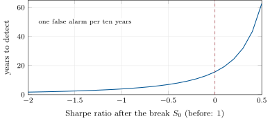
The bound is Lorden’s (1971) result, cited in omsources; the CUSUM test itself is One Quant Book 7’s (chapter 13). Its arithmetic is the chapter’s central fact. A Sharpe ratio that falls from 1 to 0, detected at one false alarm per ten years ( days), takes years to detect on average; at one per five years, 14.3. A fall to takes 3.9 years and a fall to , 1.7 (Figure 8.1). An edge that disappears quietly cannot be distinguished from bad luck on its P&L in any useful time; only an edge that turns into a loss can.
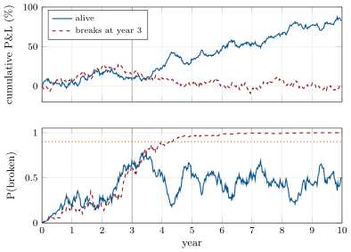
fm_drawdown.lorden.The posterior of Proposition 8.3, run on two example paths, shows what the head of desk sees (Figure 8.2). The live strategy’s posterior wanders, reaching 0.80 in its fourth year; the broken strategy’s climbs slowly after its break at the start of year four and passes 0.9 only in its fifth year.
fm_drawdown.examples.8.4 Comparing the rules
The chapter’s evaluation runs 2 000 live strategies and 2 000 that break at the start of year 4 to a Sharpe ratio of 0, for ten years, under each rule, with every stop permanent. It reports false stops per hundred live strategy-years, the share of broken strategies stopped after their break and the median delay, and the value kept per strategy over ten years: P&L less a capital charge of 2% of capital for each year run at full size (a 15% hurdle on capital of 13% of the strategy’s size), in per cent of capital.
| rule | false stops | broken | median | value, | value, | value, |
| per 100 years | caught | delay (years) | live | broken | half each | |
| none | – | – | – | 79.0 | 11.1 | 45.1 |
| stop-loss 10% | 9.79 | 34% | 0.72 | 21.7 | 15.0 | 18.3 |
| ladder 7.5 / 12.5% | 2.09 | 60% | 2.79 | 39.5 | 12.8 | 26.2 |
| time stop 18 months | 6.19 | 80% | 2.00 | 54.6 | 19.5 | 37.1 |
| posterior above 0.9 | 2.84 | 95% | 2.68 | 71.4 | 18.2 | 44.8 |
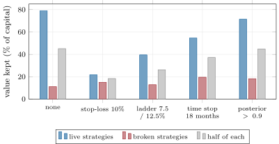
fm_drawdown.table.The 10% stop-loss is the worst rule by far. It stops 98% of healthy strategies at some point in ten years, and two thirds of the broken ones before they break; it keeps 18.3% of capital per strategy against 45.1% for no rule at all. The posterior rule stops 28% of healthy strategies over ten years, catches 95% of the broken ones about two and a half years after the break, and keeps 44.8%, as much as doing nothing. Stopping a broken strategy whose Sharpe ratio is zero saves no P&L in expectation; it saves the capital it ties up and the risk it adds, which is why the capital charge is in the value. With a charge of zero no rule beats doing nothing; with a strategy that turns into a loser, every rule catches it sooner and the posterior rule is clearly best (exercise 7).
Method 8.5 (Reviewing a strategy in drawdown)
- Express the drawdown and its duration in units of the strategy’s volatility; compare them with the distribution for a healthy strategy.
- Update the posterior that it has broken from its whole P&L history, with a hazard set from the firm’s experience of how long strategies live (One Quant Book 11, chapter 28).
- Look for evidence that is not P&L: capture and fill rates, crowding measures (One Quant Book 7, chapter 28), a change in the market’s structure. These separate bad luck from broken far faster than P&L does.
- Cut size gradually as evidence accumulates; stop only on the posterior or on non-P&L evidence; never on depth alone.
8.5 Restart, re-underwrite, retire
Definition 8.6 (Restart rule)
A restart rule states when and at what size a stopped strategy may trade again: after a fixed period, after its paper P&L recovers, or after a review of its thesis finds it intact.
A stop is a decision under uncertainty; a restart rule is what makes it reversible. Because a healthy strategy is stopped by any rule that catches broken ones in useful time, the cost of false stops is paid in the months the strategy is flat. A restart rule that paper-trades a stopped strategy and brings it back at reduced size when its paper P&L recovers recovers much of that cost; a restart that happens automatically at the new year, as in the model of One Quant Book 8, chapter 28, recovers it only for the good strategies and restarts the dead ones too. Re-underwriting a strategy is reviewing it as if it were new: its thesis, its evidence, its capacity and its cost of capital. A strategy that fails that review is retired even if its P&L has not yet said so, the only way to beat the delays of Proposition 8.4.
Remark 8.7 (The people in a drawdown)
A portfolio manager in drawdown faces rules that are public and asymmetric: a stop ends the job, a recovery restores the payout only above the high-water mark (chapter 3). Both push towards taking more risk to recover quickly or less to avoid the stop. A ladder that cuts size before the stop, and a restart rule that does not end a career at the first stop, reduce the incentive to gamble for resurrection; so does a firm that is known to review theses, not only P&L.
8.6 Tutorial: two thousand strategies and four rules
Goal. Measure what each drawdown rule costs a healthy strategy and saves on a broken one. End state: the table of rules and Figure 8.3.
- Paths.
fm_drawdown.population()draws 2 000 live and 2 000 breaking strategies withfirm.ddrules.paths. - Posterior.
firm.ddrules.posteriorruns the filter of Listing 8.1 on every path. - Rules.
fm_drawdown.table()applies the four rules withapplyand scores them withevaluate. - The bound.
fm_drawdown.lorden(10, S0)evaluates Proposition 8.4.
What to change next. Break the strategies to a Sharpe ratio of (exercise 7); set the hazard ten times too high and watch the posterior rule stop healthy strategies.
8.7 Build: drawdown rules
Purpose. Rules for managing strategies in drawdown, and an honest measure of what each costs and saves.
Interface. firm.ddrules: paths(n, days, sr, vol, rng, break_day, sr_dead); posterior(returns, sr, sr_dead, vol, hazard); Rule(kind, a, b) with kinds stop, ladder, time, posterior; apply; evaluate(rule, alive, dead, break_day, post_alive, post_dead, charge); cusum_delay(sr, sr_dead, arl_days).
Rules. A day’s size is decided on the P&L up to the day before; stops are permanent in the evaluator; value deducts the capital charge only while the strategy runs.
Acceptance tests. code/firm/ddrules/tests/: each rule on a hand-made path (the stop day, the halving, the time stop); the posterior separates live from broken populations; the evaluator’s shape; the delay formula.
Stretch. Restart rules in the evaluator; a posterior over the post-break Sharpe ratio instead of a fixed ; evidence from fill rates and capture as a second observation stream.
Sources and further reading
- M. Magdon-Ismail, A. F. Atiya, A. Pratap and Y. S. Abu-Mostafa, “On the maximum drawdown of a Brownian motion”, Journal of Applied Probability 41(1), 2004.
- G. Lorden, “Procedures for reacting to a change in distribution”, Annals of Mathematical Statistics 42(6), 1971.
- R. P. Adams and D. J. C. MacKay, “Bayesian online changepoint detection”, arXiv:0710.3742, 2007.
8.8 Exercises
Exercise 8.1 ★
Express a drawdown of 8% in years of volatility for strategies with volatilities of 10% and 30%.
Solution
Solution of Exercise 8.1.
0.8 of a year’s volatility at 10%; 0.27 at 30%.
Exercise 8.2 ★
Use Proposition 8.4 to compute the delay to detect a fall of the Sharpe ratio from 1 to 0 at one false alarm per ten years, and from 1 to .
Solution
Solution of Exercise 8.2.
days: years; to : years.
Exercise 8.3 ★
From the table of rules, what share of healthy strategies does the 10% stop-loss stop over ten years, and what share of broken ones does it stop before they break?
Solution
Solution of Exercise 8.3.
of healthy strategies over ten years; 66% of broken ones before their break.
Exercise 8.4 ★★
A strategy’s posterior of having broken is 0.30 and the daily hazard is . Its next day’s return is exactly the broken mean. Is the posterior higher or lower after that day, and why does one day move it so little?
Solution
Solution of Exercise 8.4.
Higher: the prior becomes , and the return favours the broken state by a likelihood ratio of only , so the posterior is 0.3010. One day’s return carries a signal of standard deviations.
Exercise 8.5 ★★
Why does stopping a broken strategy whose Sharpe ratio is zero add no expected P&L, and what does it save?
Solution
Solution of Exercise 8.5.
Its expected P&L is zero after the break, so stopping it forgoes nothing and gains nothing in expectation. It frees the capital and the risk it uses: the capital charge while it runs, and the variance it adds to the firm.
Exercise 8.6 ★★
A strategy has a Sharpe ratio of 1 and a volatility of 10%. Its maximum drawdown over ten years has a median of 16.8%. Is a 12% drawdown in its sixth year evidence that it has broken?
Solution
Solution of Exercise 8.6.
No: 12% is below the median ten-year maximum drawdown of a healthy strategy (16.8%); drawdowns of that depth are normal and say little about a break.
Exercise 8.7 ★★★
Coding. Rerun the evaluation with broken strategies falling to a Sharpe ratio of (set SR_DEAD and the posterior’s alternative to ). What happens to the delays and to each rule’s value?
Solution
Solution of Exercise 8.7.
The posterior rule catches broken strategies after a median 1.3 years (false stops 2.24 per hundred years); values for a half-and-half population are 17.5 (stop-loss), 23.2 (ladder), 31.3 (time stop) and 39.3 (posterior) against 10.1 with no rule. When a break turns into losses, every rule helps and the posterior rule most.
Exercise 8.8 ★★★
Find the flaw. “We backtested our 10% stop-loss on our strategies’ histories and it would have avoided every large loss. Adopt it.”
Solution
Solution of Exercise 8.8.
The backtest counts the losses avoided and not the recoveries forgone: the stop fires on healthy strategies in ordinary drawdowns (98% of them over ten years in the chapter’s model). Count false stops and the P&L lost after them, on strategies known to be healthy, before adopting it.
8.9 Problem: Down Eight in March
Problem 8.1
Weekend problem — down eight in March
Two portfolio managers are each down 8% from their peak. The head of desk must decide what to do with each, and what rule to adopt for next time.
Part I — The drawdown.
- Define a stop-loss rule, a de-risking ladder and a time stop.
- Give the median and 90th percentile of a healthy Sharpe-1 strategy’s maximum drawdown over ten years at 10% volatility.
- Express 8% in volatility units for both managers, at 10% and 20% volatility.
- Why do thresholds belong in volatility units?
Part II — The evidence.
- State and prove Proposition 8.3.
- Give the mean posterior on the day a healthy and a broken strategy first reach an 8% drawdown.
- State Proposition 8.4 and compute the delay for a fall from 1 to 0 and to at one false alarm per ten years.
- Which kinds of evidence separate bad luck from broken faster than P&L?
Part III — The rules.
- Give each rule’s false stops per hundred strategy-years and the share of broken strategies caught after their break.
- Give each rule’s median detection delay.
- Give each rule’s value kept for live, broken and mixed populations, against no rule.
- Why is the stop-loss the worst rule?
- Why does the posterior rule keep about as much as no rule, and when would it keep more?
Part IV — The decision.
- Define a restart rule and describe a good one.
- What is re-underwriting, and why can it beat the delays of the P&L?
- What do the rules do to a portfolio manager’s incentives in drawdown?
- What would you do with each of the two managers on Monday?
- Which rule would you adopt, with which thresholds, and why?
- State the named result: the posterior on the day of the 8% drawdown for a healthy and a broken strategy, and the detection delay of a fall from 1 to 0 at one false alarm per ten years.
- In two sentences, explain to the managers how they will be judged.
Solution
Solution of Problem 8.1.
- See Definition 8.2.
- 16.8% and 25.4% of capital.
- 0.8 and 0.4 of a year’s volatility.
- A healthy strategy’s drawdowns scale with its volatility; a threshold in per cent means different things for different strategies.
- See Proposition 8.3.
- 0.24 for healthy strategies and 0.39 for broken ones (only 13% of broken paths first reach 8% after their break).
- Delay years: 15.7 and 3.9.
- Capture and fill rates, crowding measures, changes in market structure: observations that move with the edge itself, not with the strategy’s noise.
- False stops 9.79, 2.09, 6.19 and 2.84 per hundred strategy-years; caught 34%, 60%, 80% and 95%.
- 0.72, 2.79, 2.00 and 2.68 years.
- Live 21.7, 39.5, 54.6, 71.4; broken 15.0, 12.8, 19.5, 18.2; half each 18.3, 26.2, 37.1, 44.8; no rule 79.0, 11.1, 45.1.
- It stops almost every healthy strategy in an ordinary drawdown, and most broken ones before they break.
- Stopping a broken strategy at Sharpe 0 saves only its capital charge; it keeps more when broken strategies lose money (exercise 7).
- See Definition 8.6: paper-trade the stopped strategy and restart at reduced size when its paper P&L recovers.
- Reviewing the strategy’s thesis and evidence as if new; it uses information other than P&L.
- They push managers to gamble for resurrection or to freeze; ladders and restart rules soften both.
- Compare both drawdowns in volatility units and with healthy distributions; look at non-P&L evidence; cut size only if it points to a break.
- The posterior rule with a hazard from the firm’s experience, a ladder for size, and a restart rule; no depth-only stop.
- Posterior 0.24 (healthy) and 0.39 (broken) at the 8% drawdown; 15.7 years to detect a fall from 1 to 0 at one false alarm per ten years.
- You will be judged on the evidence that your edge is intact, of which your drawdown is a weak part; your size will fall gradually as evidence against it builds, and a stop will not be the end if the evidence recovers.
8.10 Interview questions
Interview question 8.1 ★ trader
Your strategy has a Sharpe ratio of 1 and 10% volatility and is 15% below its peak. Should you be worried?
Solution
Solution of Interview question 8.1.
Not by itself: 15% is 1.5 years’ volatility, within the normal range of a Sharpe-1 strategy’s ten-year maximum drawdown (median about 17%).
What the interviewer is looking for: volatility units and the healthy distribution.
Interview question 8.2 ★ risk
What is the difference between a stop-loss and a de-risking ladder, and why might a firm prefer the ladder?
Solution
Solution of Interview question 8.2.
A stop ends trading at one threshold; a ladder cuts size in steps. The ladder has fewer false stops and responds before the stop.
What the interviewer is looking for: graduated response.
Interview question 8.3 ★★ researcher
How long would it take to detect, from daily P&L, that a strategy’s Sharpe ratio has fallen from 1 to 0? Derive the order of magnitude.
Solution
Solution of Interview question 8.3.
KL per day ; delay days, about 16 years at .
What the interviewer is looking for: information per day and log of the false-alarm period.
Interview question 8.4 ★★ researcher, risk
Write the update of the probability that a strategy has broken, given one more day of returns.
Solution
Solution of Interview question 8.4.
Predict , then Bayes with the two Gaussian likelihoods (Proposition 8.3).
What the interviewer is looking for: the prediction and update steps.
Interview question 8.5 ★★ trader, risk
A backtest shows that a stop-loss would have avoided every large loss. What would you check?
Solution
Solution of Interview question 8.5.
How often it would have stopped strategies that went on to recover, and what those recoveries were worth.
What the interviewer is looking for: false stops and forgone recoveries.
Interview question 8.6 ★★★ researcher
Your P&L cannot tell you in time whether an edge has gone. What else would you monitor, and why is it faster?
Solution
Solution of Interview question 8.6.
Capture, fill and hit rates, signal decay, crowding and flows: they measure the edge directly, with far less noise per day than P&L.
What the interviewer is looking for: higher signal-to-noise observations.