The Desk and the Firm · The firm
9Managing Researchers, Traders and Engineers
Three researchers’ signals went into one combined forecast that made $30 million in a year. Asked what each had contributed, the desk measured what the forecast would have lost without each signal in turn: $2.5 million, $2.7 million and $4.6 million, less than a third of the profit between them. Two of the signals were two routes to the same effect, so each looked nearly worthless once the other was there. The rest of the $30 million had to be split some other way, and the way it was split decided which of the three stayed.
9.1 Choosing projects: a research portfolio
A quantitative desk spends much of its budget on work whose value is uncertain: new signals, new markets, new models, better execution. The head of desk chooses among projects as an investor chooses among assets, with the same two questions: what is each expected to return, and how do the returns combine.
Definition 9.1 (Research portfolio, project scorecard)
A desk’s research portfolio is the set of research and development projects it funds in a period, chosen under a budget of money and people. A project scorecard records each candidate’s cost, probability of success, value if it succeeds (the present value of the P&L it adds, net of its running costs), its overlap with what the desk already runs, and the evidence behind each estimate.
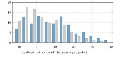
A project’s expected net value is . The chapter’s desk has twelve candidates (illustrative, $ million): a new futures signal (cost 1.5, probability 0.30, value 12), options-flow features (2.0, 0.20, 15), an execution model (1.0, 0.60, 4), an alternative-data trial (2.5, 0.10, 20), a second momentum variant that overlaps the book by 70% (1.0, 0.40, 6), and seven others. With a budget of $10 million, choosing greedily by expected net value per dollar of cost funds six projects with an expected net value of $8.15 million. Over 20 000 simulated years the chosen portfolio returns $8.08 million on average and loses money in 28.5% of years; a portfolio chosen at random within the same budget returns $3.65 million and loses in 44.8% (Figure 9.1).
fm_research.portfolio_samples.Remark 9.2 (The scorecard’s weak inputs)
The probabilities of success are the weakest numbers on a scorecard and the most important. They come from the desk’s own history (how many of its past projects of each kind reached production, which the research log of One Quant Book 7, chapter 1 records) and they are optimistic when they come from the proposer. Keeping the history is what turns the portfolio from a debate into an estimate.
9.2 Review without theatre
A research review (One Quant Book 7, chapter 1) is where a project meets its evidence. Reviews become theatre when their outcome does not depend on what is presented: when the project’s sponsor is senior, when the backtest is shown without the number of variants tried, when a kill criterion was never written. The procedures that prevent it are already in the series: pre-registration of the hypothesis and of the test, a trial count kept in the research log, stage gates with kill criteria agreed before the evidence arrives.
Method 9.3 (A review that decides)
- Before the work: record the hypothesis, the test, the kill criterion and the stage gate in the research log.
- At the review: present the result against the pre-registered test, with the number of trials run and the deflated Sharpe ratio (One Quant Book 4, chapter 12).
- Decide by the gate: proceed, stop or change the hypothesis, which starts a new trial count.
- Review the reviewers once a year: compare their decisions with what reached production and what it earned.
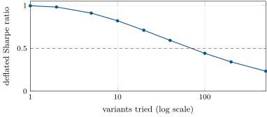
The trial count matters more than any other number in the review. A backtest with a Sharpe ratio of 1.2 over five years of daily data has a probabilistic Sharpe ratio of 0.996: taken alone, it is almost certainly real. If it is the best of 40 variants tried, the expected best of 40 worthless variants (with a spread of Sharpe ratios of 0.5 a year) is 1.09, and the deflated Sharpe ratio falls to 0.59 (Figure 9.2). The same result, after 200 variants, is more likely luck than skill.
fm_research.dsr_curve, on One Quant Book 4’s firm.multitest.9.3 Who made the money: attributing credit
Definition 9.4 (Leave-one-out contribution, credit attribution)
A contributor’s leave-one-out contribution to a combined result is the result with every contributor less the result without that contributor. Credit attribution is a rule that splits a combined result among the contributors to it, and on which their recognition and pay are based.
A combined forecast is a game in the sense of the Shapley value (One Quant Book 12, chapter 6): each set of contributors has a worth , the P&L of the best combination of their signals. Leave-one-out credit, , measures what each adds last; when two contributors bring the same information, each adds little last and both look worthless. Order-dependent credit gives each contributor what they added when they arrived, so the first of two overlapping signals gets everything and the second nothing. The Shapley value averages the order over all orders.
Proposition 9.5 (What the Shapley split guarantees)
The Shapley value , the average over orders of what adds to the set of contributors before it, satisfies ; gives equal credit to contributors who add the same to every set; and gives nothing to a contributor who adds nothing to any set. Leave-one-out credit satisfies the last two but in general not the first: when contributions are substitutes, summed over is less than .
Partial proof. For each order the added values telescope to ; averaging preserves the sum. Symmetric contributors have identical distributions of added values over orders; a contributor who adds nothing adds nothing in every order. For leave-one-out, take two identical contributors: each adds nothing last, so both get zero while . That the Shapley value is the only rule with these properties and additivity across games is Shapley’s theorem (1953), cited in omsources. ∎
def leave_one_out(v, n: int) -> np.ndarray:
    full = frozenset(range(n))
    return np.array([v(full) - v(full - {i}) for i in range(n)])


def ordered(v, order) -> np.ndarray:
    out = np.zeros(len(order))
    seen = set()
    for i in order:
        before = v(seen)
        seen.add(i)
        out[i] = v(seen) - before
    return out


def shapley(v, n: int, samples: int | None = None, rng=None) -> np.ndarray:
    if samples is None:
        tot = np.zeros(n)
        for order in itertools.permutations(range(n)):
            tot += ordered(v, order)
        return tot / math.factorial(n)
    tot = np.zeros(n)
    for _ in range(samples):
        tot += ordered(v, list(rng.permutation(n)))
return tot / samplesIn the chapter’s desk (illustrative: signals A and B correlated at 0.8, C independent, ten years of daily data, the combined P&L scaled to $30 million), the rules disagree completely (Figure 9.3):
| contributor | alone | leave-one-out | order A, B, C | Shapley |
|---|---|---|---|---|
| A | 22.77 | 2.46 | 22.77 | 12.63 |
| B | 22.84 | 2.67 | 2.59 | 12.77 |
| C | 4.55 | 4.64 | 4.64 | 4.61 |
| sum | – | 9.77 | 30.00 | 30.00 |
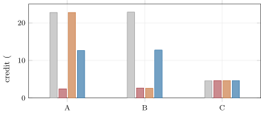
fm_research.credit.A bonus pool of $6 million split in proportion to each rule’s credits gives A, B and C $1.51, $1.64 and $2.85 million by leave-one-out, $2.53, $2.55 and $0.92 million by Shapley, and $4.55, $0.52 and $0.93 million by order of arrival. Leave-one-out pays C most, because C is the only one whose signal cannot be replaced; order of arrival pays whoever came first. Shapley pays A and B as a pair for the effect they both found, and C for what only C found. The credits are themselves estimates: rerun on another ten years of data (exercise 7), the split moves by several million.
9.4 Keeping research honest
Credit rules shape research as much as they measure it. Paid by leave-one-out, researchers avoid overlapping work, including the replication that would expose a spurious signal; paid by order of arrival, they race to be first and hoard; paid by stand-alone P&L, they rediscover what the book already holds. Paid by Shapley, a researcher who finds a second route to an effect the desk already exploits is paid for part of it, which rewards robustness and replication. Three further rules keep research honest whatever the credit rule: every trial goes in the research log; results are presented against a pre-registered test; and the people who review a signal are not those who are paid for it.
9.5 Traders and engineers: different work, different feedback
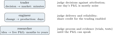
Researchers, traders and engineers get feedback at different speeds, and managing them the same way fails all three (Figure 9.4). A trader sees the market’s verdict in minutes and must be judged on decisions, not only on the day’s P&L, whose noise dominates it: attribution of P&L to risk taken and to execution (One Quant Book 1, chapter 7) is the tool. A researcher’s work pays off, if ever, after months of testing and years of live trading: the measure is the quality of the process, trials and evidence, until the P&L can speak. An engineer’s work shows in systems that run or do not: delivery, reliability and the time it takes to restore service are measured daily (One Quant Book 15, chapter 28), and the value of the work is the trading it enables, which is why engineers belong in the credit attribution of the strategies they make possible.
9.6 Tutorial: a year of research, and the credit for it
Goal. Choose a research portfolio, deflate a result by its trials, and split the credit for a combined forecast. End state: the credit table and Figure 9.3.
- The portfolio.
firm.projsel.select(fm_research.PROJECTS, 10)chooses six projects;fm_research.portfolio()simulates 20 000 years of the choice and of random choices. - The trials.
fm_research.deflated(trials=40)gives the probabilistic and deflated Sharpe ratios of a five-year backtest with a Sharpe ratio of 1.2. - The game.
firm.projsel.game(signals, target)builds ;leave_one_out,orderedandshapleysplit it (Listing 9.1). - The pool.
fm_research.pool_split()turns each rule’s credit into shares of a $6 million pool.
What to change next. Make A and B identical and check that Shapley pays them equally and leave-one-out pays them nothing; rerun on another seed and measure how uncertain each credit is.
9.7 Build: research portfolio and credit
Purpose. The head of desk’s two allocation problems: which projects to fund, and how to credit the people whose work combined.
Interface. firm.projsel: Project(name, cost, p, value, overlap), expected_net; select(projects, budget), select_random, simulate_year; game(signals, target); leave_one_out, ordered, shapley(v, n, samples, rng). The chapter uses One Quant Book 4’s firm.multitest for deflated Sharpe ratios.
Rules. Projects with non-positive expected net value are never funded; the game’s worth is the in-sample P&L of the least-squares combination; exact Shapley values for up to about eight contributors, sampled beyond.
Acceptance tests. code/firm/projsel/tests/: greedy selection within the budget; Shapley efficiency, symmetry of identical contributors and zero for a dummy; leave-one-out zero for a duplicated contributor; sampled Shapley close to exact.
Stretch. Out-of-sample games (the worth of measured on data not used to fit the weights); a portfolio with correlated project outcomes; credit with a time dimension (who kept a signal alive).
Sources and further reading
- L. S. Shapley, “A value for n-person games”, in Contributions to the Theory of Games II, 1953.
- S. Lipovetsky and M. Conklin, “Analysis of regression in game theory approach”, Applied Stochastic Models in Business and Industry 17(4), 2001.
- D. H. Bailey and M. López de Prado, “The deflated Sharpe ratio”, Journal of Portfolio Management 40(5), 2014.
- C. R. Harvey, Y. Liu and H. Zhu, “… and the cross-section of expected returns”, Review of Financial Studies 29(1), 2016.
9.8 Exercises
Exercise 9.1 ★
The new futures signal costs $1.5 million, succeeds with probability 0.30 and is then worth $12 million. What is its expected net value, and per dollar of cost?
Solution
Solution of Exercise 9.1.
million; 1.4 per dollar of cost.
Exercise 9.2 ★
The second momentum variant costs $1.0 million, succeeds with probability 0.40, is worth $6 million and overlaps the book by 70%. Should it be funded?
Solution
Solution of Exercise 9.2.
million: no; most of its value is already in the book.
Exercise 9.3 ★
Check that the Shapley credits of the table add up to the combined P&L, and compute what leave-one-out leaves unallocated.
Solution
Solution of Exercise 9.3.
; leave-one-out allocates 9.77 and leaves $20.23 million unallocated.
Exercise 9.4 ★★
Two contributors bring identical signals worth 20 alone and 20 together; a third brings an independent signal worth 10. Compute the leave-one-out and Shapley credits.
Solution
Solution of Exercise 9.4.
Leave-one-out: 0, 0 and 10. Shapley: 10, 10 and 10: the two identical contributors share the 20 their effect is worth, and the third gets its own 10.
Exercise 9.5 ★★
From Figure 9.2, after how many variants does the chapter’s backtest fall below an even chance of beating luck?
Solution
Solution of Exercise 9.5.
At about 70 variants (0.59 at 40, 0.44 at 100).
Exercise 9.6 ★★
Which credit rule rewards a researcher for replicating a signal the desk already trades, and why is that valuable?
Solution
Solution of Exercise 9.6.
Shapley: it gives a second route to a known effect part of that effect’s credit. Replication confirms that the effect is real and survives a different implementation, which is how spurious signals are found.
Exercise 9.7 ★★★
Coding. Rerun fm_research.credit(seed=12). How do the leave-one-out and Shapley credits change, and what does that say about paying on one year’s attribution?
Solution
Solution of Exercise 9.7.
Leave-one-out becomes 1.0, 2.7 and 13.0; Shapley 7.8, 9.5 and 12.7. On one sample the credits move by several million: pay on attribution averaged over years, or on process as well as attribution.
Exercise 9.8 ★★★
Find the flaw. “We pay each researcher 10% of what the desk would lose if their signal were switched off. That is fair: it is exactly what they add.”
Solution
Solution of Exercise 9.8.
Leave-one-out credits do not add up to the desk’s P&L when signals overlap, so overlapping researchers are paid almost nothing for real work, and a desk that pays only on them discourages replication. The Shapley value adds up and treats substitutes symmetrically.
9.9 Problem: Who Made the Money
Problem 9.1
Weekend problem — who made the money
A combined forecast made $30 million. Three researchers ask for their share of a $6 million pool, and the head of desk must also fund next year’s research.
Part I — The portfolio.
- Define a research portfolio and a project scorecard.
- Which six projects does the greedy rule fund, and at what expected net value?
- Give the mean realised value and the probability of a losing year for the greedy and the random choices.
- Where do the probabilities of success on a scorecard come from, and why are they optimistic?
Part II — The review.
- What makes a review theatre, and what prevents it?
- Give the probabilistic and the deflated Sharpe ratio of the five-year backtest after 40 variants.
- What is the expected best Sharpe ratio of 40 worthless variants?
- Why must a new hypothesis start a new trial count?
Part III — The credit.
- Define leave-one-out contribution and credit attribution.
- Give each researcher’s credit alone, by leave-one-out, by order of arrival and by Shapley.
- State Proposition 9.5 and prove its first part.
- Why does leave-one-out leave most of the profit unallocated here?
- Split the $6 million pool by leave-one-out, Shapley and order of arrival.
- How uncertain are these credits?
Part IV — The people.
- What does each credit rule encourage researchers to do?
- How should traders and engineers be judged while their results are noise?
- Why do engineers belong in a strategy’s credit attribution?
- Who should review a signal, and who should not?
- State the named result: the Shapley and leave-one-out credits of the three researchers, and the pool split each implies.
- In two sentences, explain to the three researchers how the pool was split.
Solution
Solution of Problem 9.1.
- See Definition 9.1.
- The execution model, the new futures signal, the auction imbalance model, the options flow features, the crypto basis book and the borrow-cost signal; $8.15 million expected, for $10 million of cost.
- Greedy $8.08 million and 28.5%; random $3.65 million and 44.8%.
- From the desk’s history of past projects of each kind; proposers are optimistic about their own.
- When the outcome does not depend on the evidence; pre-registration, trial counts and agreed kill criteria.
- 0.996 and 0.59.
- 1.09 a year.
- The old trials were chosen with the old hypothesis; a new one is tested afresh and its search counted afresh.
- See Definition 9.4.
- Alone 22.77, 22.84, 4.55; leave-one-out 2.46, 2.67, 4.64; order A, B, C 22.77, 2.59, 4.64; Shapley 12.63, 12.77, 4.61.
- Each order’s added values telescope to ; their average does too.
- A and B are substitutes: each adds almost nothing once the other is there.
- Leave-one-out 1.51, 1.64, 2.85; Shapley 2.53, 2.55, 0.92; order 4.55, 0.52, 0.93 ($ million).
- Very: on another ten years of data they move by several million each.
- Leave-one-out: avoid overlap and replication; order: race and hoard; stand-alone: rediscover the book; Shapley: work on robust effects.
- Traders on decisions and attribution; engineers on delivery and reliability; both over periods long enough for noise to average out.
- Their systems are part of the strategy’s edge: the P&L depends on them.
- People who are not paid for it.
- Shapley 12.63, 12.77 and 4.61; leave-one-out 2.46, 2.67 and 4.64; pool splits $2.53, 2.55, 0.92 million and $1.51, 1.64, 2.85 million.
- A and B found the same effect by two routes and share the credit for it; C found an effect no one else did and is paid all of it. The split is the average of what each added in every possible order of arrival.
9.10 Interview questions
Interview question 9.1 ★ researcher
Two of your signals are highly correlated. What happens to each one’s leave-one-out contribution to the combined forecast?
Solution
Solution of Interview question 9.1.
Both become small: each adds little once the other is in the forecast.
What the interviewer is looking for: substitution between correlated signals.
Interview question 9.2 ★ researcher
Your backtest has a Sharpe ratio of 1.2 over five years. What else do you need to say before anyone should believe it?
Solution
Solution of Interview question 9.2.
How many variants were tried, the deflated Sharpe ratio, the costs assumed, and whether the test was pre-registered.
What the interviewer is looking for: trial count and deflation.
Interview question 9.3 ★★ researcher, trader
Define the Shapley value and give one property that leave-one-out credit lacks.
Solution
Solution of Interview question 9.3.
The average over orders of each contributor’s added value; its credits add up to the total, which leave-one-out credits do not.
What the interviewer is looking for: the definition and efficiency.
Interview question 9.4 ★★ developer
How would you measure an engineering team’s contribution to a trading desk?
Solution
Solution of Interview question 9.4.
Delivery and reliability metrics for the work, and a share of the credit for the strategies the systems enable, measured by what the desk could not trade without them.
What the interviewer is looking for: outcomes enabled, not lines of code.
Interview question 9.5 ★★ researcher
You have a budget for five projects out of twelve. How do you choose, and which input do you trust least?
Solution
Solution of Interview question 9.5.
Rank by expected net value per unit of cost, adjust for overlap and diversification; the probabilities of success are the least reliable input.
What the interviewer is looking for: a scorecard and humility about probabilities.
Interview question 9.6 ★★★ researcher
Computing exact Shapley values needs orders. How would you attribute credit among 30 contributors?
Solution
Solution of Interview question 9.6.
Sample random orders (Monte Carlo Shapley), or group contributors and compute Shapley values between groups and within them.
What the interviewer is looking for: sampling or hierarchical approximation.