1Why Financial Machine Learning Is Different

A new model forecasts next month’s return of 500 stocks. Out of sample, over ten years, its R-squared is 0.57%, and the desk is pleased. It should be: in the simulated market the model was trained on, where the expected returns are known because they were planted, the best forecast that can exist scores 0.60%. The same gradient-boosted trees, given a task whose signal is strong, explain 92% of the variance. Nothing is wrong with either number. The model did as well on the stocks as it did on the easy task; the stocks simply contain almost nothing to learn, and what they contain changes, is shared by every stock at once, and is traded away by whoever learns it first. This chapter fixes the vocabulary of machine learning the rest of the book uses, and measures, on data whose truth is known, the four ways market data differ from the data the field grew up on.

1.1 Learning from data: the vocabulary

Definition 1.1 (Supervised and unsupervised learning)

Supervised learning fits a function $f_\theta$ from features $x\in\mathbb R^p$ to a target $y$ on examples $(x_i, y_i)$, $i = 1,\dots,n$, by minimising an empirical loss $\mathcal L_n(\theta) = \frac1n\sum_i\ell(y_i, f_\theta(x_i))$, so that $f_\theta$ predicts $y$ for new $x$. Unsupervised learning has no target: it describes the distribution of $x$ itself (clusters, factors, a lower-dimensional representation, a density).

The target is Book 7’s prediction target (chapter 6): a forward return over a forecast horizon, or a label built from one (chapter 2 of this book). The loss $\ell(y,\hat y)$ always takes two arguments here; $\mathcal L_n$ is always subscripted. The learning rate of later chapters is written $\eta$, a symbol declared local to this book (the series keeps $\eta$ for the vol-of-vol elsewhere).

Definition 1.2 (Training, validation and test sets; hyperparameter)

The training set is the data on which $\theta$ is fitted. A hyperparameter is a choice the fit does not make itself (a penalty, a tree depth, a number of layers, a learning rate); the validation set is data held out from the fit on which hyperparameters are chosen. The test set is data used once, after every choice is made, to estimate how the chosen model will perform.

On market data the three sets are consecutive stretches of time, in that order (Figure 1.1), because the model will be used on a future it has not seen. The test set is Book 7’s holdout set (chapter 1): touched once. A test set consulted twice has become a validation set.

Definition 1.3 (Generalisation error, overfitting, bias–variance decomposition)

The generalisation error of a fitted model $\hat f$ is its expected loss on a new draw $(x, y)$ from the distribution the model will meet. Overfitting is the fitting of features of the training sample that do not recur, so that the in-sample loss understates the generalisation error. For the squared loss, the bias–variance decomposition splits the expected generalisation error at a point into noise, squared bias and variance (Proposition 1.4).

Proposition 1.4 (Bias–variance decomposition)

Let $y = \mu(x) + \varepsilon$ with $\E[\varepsilon\mid x] = 0$ and $\Var(\varepsilon\mid x) = \sigma^2(x)$, and let $\hat f$ be fitted on a training sample independent of $(x, y)$. Then

$$\E\bigl[(y - \hat f(x))^2 \bigm| x\bigr] = \sigma^2(x) + \bigl(\E[\hat f(x)] - \mu(x)\bigr)^2 + \Var\bigl(\hat f(x)\bigr),$$

where $\E$ and $\Var$ of $\hat f(x)$ are over training samples.

The noise $\sigma^2$ is the floor no model goes below. In most of machine learning the noise is small and the fight is between bias (a model too rigid for $\mu$) and variance (a model that follows the sample). On market data $\sigma^2$ is almost all of the loss, and a model with any variance at all spends it on noise: the balance tips towards rigid, regularised models (chapter 4).

1.2 Signal-to-noise near zero and the R-squared ceiling

Definition 1.5 (Out-of-sample R-squared, predictability ceiling)

The out-of-sample R-squared of forecasts $\hat y_i$ of returns $y_i$ on a test set is

$$R^2_{\mathrm{oos}} = 1 - \frac{\sum_i(y_i - \hat y_i)^2}{\sum_i y_i^2},$$

measured against a forecast of zero, not against the sample mean. The predictability ceiling of a dataset is $R^2_{\mathrm{oos}}$ of the true conditional expectation $\mu(x_i) = \E[y_i\mid x_i]$: the best any model of those features can score.

The zero benchmark follows Gu, Kelly and Xiu, whose study of 30 000 stocks over 60 years uses it because the historical mean of a stock’s return is so noisy a forecast that beating it is too easy. Their monthly out-of-sample stock-level R-squared runs from 0.16% for a three-variable linear model to 0.33–0.40% for trees and neural networks, with 0.40% for the best network. Those are the numbers of a field where half a per cent is a strong result.

Proposition 1.6 (The ceiling bounds every model; R-squared and correlation)

1. For any forecast $\hat f(x)$ built from the features, $\E(y - \hat f)^2 \ge \E(y - \mu)^2$: in expectation, no model’s $R^2_{\mathrm{oos}}$ exceeds the ceiling.
2. If $y$ and a forecast $f$ have mean zero, $\operatorname{Corr}(f, y) = \rho$, and the forecast is used as $c f$, then $R^2_{\mathrm{oos}}(c) = (2c\rho\sigma_y\sigma_f - c^2\sigma_f^2)/\sigma_y^2$, maximal at $c^\star = \rho\sigma_y/\sigma_f$ where it equals $\rho^2$, and zero at $c = 2c^\star$.

The second part links R-squared to the information coefficient of Book 7 (chapter 6): a forecast whose correlation with returns is $\rho$ earns at most $\rho^2$, and a correlation of 0.075 is an R-squared of 0.56%. It also says how a good forecast scores badly: a forecast with the right direction and twice the right size scores zero.

The book’s sandbox, firm.mlsynth, draws a monthly cross-section of 500 stocks with twenty characteristics published as cross-sectional ranks in $[-1, 1]$, as the empirical literature ranks them. Six carry signal, linearly and through an interaction, a square, a threshold and an absolute value; fourteen are noise. Returns add a market factor, ten industry factors and heavy-tailed specific shocks, and the planted expected return is scaled so that the ceiling is 0.7%. Ridge regression, LightGBM’s gradient-boosted trees and a small multilayer perceptron are trained on twenty years and tested on the next ten (Table 1.1); for comparison, the same three models are fitted to a task with a Bayes-optimal R-squared of 0.95 (20 000 examples, a smooth nonlinear function of five of twenty features).

	500 stocks, ceiling 0.60% out of sample			strong signal, Bayes 0.95
model	in sample	out of sample	corr. with the truth	in sample	out of sample
ridge regression	0.39%	0.38%	0.74	0.72	0.72
boosted trees	1.45%	0.57%	0.92	0.92	0.92
neural network	0.64%	0.28%	0.74	0.94	0.93

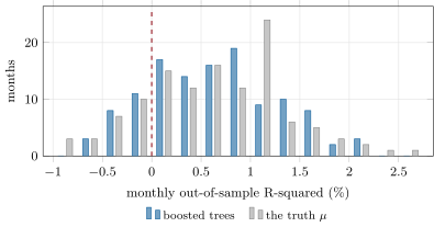
Table 1.1 is the chapter in miniature. On the strong task every model’s in-sample and out-of-sample scores agree and the flexible models win. On the stocks, the boosted trees’ in-sample R-squared is 1.45%, twice the ceiling of the training years (0.72%): the excess is noise it has fitted. Its out-of-sample 0.57% is 95% of the ceiling, the best of the three; the linear model reaches 64% of it, and the network, trained here without the care of chapter 7, less than half. The forecasts’ correlations with the truth (0.74 to 0.92) are high; their correlations with the realised returns are below 0.08.

1.3 Non-stationarity and adversarial feedback

The distribution a model meets is not the one it was trained on. Some change is exogenous (a new regulation, a new venue, a crisis). Some is caused by the model’s own trade and its competitors’: a predictor that is public, or that several firms have found, is traded until its return is smaller than its cost. Book 7 measured the result on real anomalies as post-publication decay (chapter 13) and its cause as crowding (chapter 28). In the physical sciences the data do not read the paper.

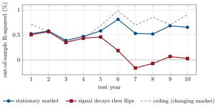
firm.mlsynth can age a signal. From the first test month the strongest linear characteristic’s effect decays with a half-life of two years, and five years into the test the interaction between two characteristics changes sign. The boosted trees, trained once on the first twenty years, keep their R-squared through the decay, which the other characteristics hide, and lose it when the interaction flips (Figure 1.3): years 6 to 10 average 0.01%, while the ceiling, which moves with the new truth, averages 0.83%. Nothing in the model’s inputs announced the change; its errors did. Chapter 12 detects it and chapter 27 builds the alarms.

1.4 Small effective samples

The training set holds $240 \times 500 = 120\,000$ stock-months. It is not 120 000 independent observations. The stocks’ unexpected returns share a market and an industry: their average pairwise correlation is 0.27, and the effective number of independent stocks in a month, $n/(1 + (n-1)\bar\rho)$, is 3.7 out of 500. Whatever depends on the market’s path is estimated from 240 draws, not 120 000.

The intercept is the clearest case. Trained on raw returns, a model’s intercept is the training window’s average market return. The true premium in the sandbox is zero; the window happened to average $-0.56\%$ a month, about two standard errors of a 240-month mean at a 4.5% monthly volatility. The three models trained on raw returns score $-0.29\%$, $-0.09\%$ and $-0.30\%$ out of sample, each of them worse than a forecast of zero. Trained on returns minus each month’s cross-sectional mean, they learn which stocks do better, not where the market goes, and score the table’s numbers.

Method 1.7 (Before fitting a model of returns)

1. Compute or bound the ceiling: on synthetic data exactly; on real data, from the best published R-squared or information coefficient of comparable work (Proposition 1.6).
2. Decide what the model is asked: the cross-section (demean or rank the target by date), or the level.
3. Count the effective sample: dates, not rows, for anything common to all assets; overlapping labels (chapter 2) divide it again.
4. Fix the test period before looking at it, and plan how long a live track must be to tell the model from zero and from the simpler model.

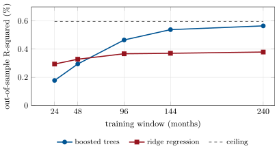
Length is the other effective sample. The boosted trees’ monthly R-squared has a mean of 0.62% and a standard deviation of 0.64%: 4.3 months of live trading put its mean two standard errors from zero. Telling it from ridge regression takes longer: the monthly difference has a mean of 0.21% and a standard deviation of 0.47%, which needs 21 months. With less history the flexible model loses its advantage (Figure 1.4): trained on the last two years only, the trees score 0.18% and ridge 0.29%; they cross between four and eight years. The more flexible the model, the more of its training data goes to learning what the noise is not.

1.5 What carries over from the rest of machine learning, and what does not

The algorithms carry over: least squares and its penalties (Book 4, chapter 16), trees, networks, gradient methods (Book 4, chapter 24). So does the discipline of held-out evaluation. What does not carry over is the default settings and the intuitions trained on images and text: shuffled cross-validation (Book 7, chapter 20, and chapter 3), a validation score read as a fact rather than a draw, hyperparameters tuned until the validation set agrees, an accuracy of 55% taken for a weak model when it may be close to the ceiling, and a model fitted once and trusted for years. Every chapter of this book is one of these corrections, measured.

1.6 Tutorial: the 0.57% model

1.7 Build: synthetic learning tasks

1.8 Exercises

Exercise 1.1 ★

A forecast of next month’s returns has a correlation of 0.05 with them and is optimally scaled. What is its out-of-sample R-squared? What if it is used at three times the optimal scale?

Solution

Solution of Exercise 1.1.

$R^2 = \rho^2 = 0.25\%$. At $c = kc^\star$, $R^2 = \rho^2(2k - k^2)$; for $k = 3$, $-3\rho^2 = -0.75\%$.

Exercise 1.2 ★

The unexpected returns of 500 stocks have an average pairwise correlation of 0.27. What is the effective number of independent stocks in a month? With 0.05?

Solution

Solution of Exercise 1.2.

$500/(1 + 499\times0.27) = 3.7$; with 0.05, $500/(1 + 24.95) = 19.3$.

Exercise 1.3 ★

A model’s monthly R-squared has a mean of 0.5% and a standard deviation of 0.8%. How many months of independent results put the mean two standard errors from zero? Three?

Solution

Solution of Exercise 1.3.

$(2\times0.8/0.5)^2 = 10.2$ months; for three standard errors $(3\times0.8/0.5)^2 = 23.0$.

Exercise 1.4 ★★

The boosted trees score 1.45% in sample, where the ceiling is 0.72%. How can a model beat the best possible predictor in sample, and what does the gap say about its out-of-sample score?

Solution

Solution of Exercise 1.4.

The ceiling is the R-squared of the truth; a model fitted to the same sample can also fit that sample’s noise, which the truth does not, so its in-sample R-squared can exceed the ceiling. The excess (0.73 points) is fitted noise: it is the variance term of Proposition 1.4 seen from inside the sample, and it will not recur. Out of sample the trees cannot beat 0.60% in expectation and score 0.57%.

Exercise 1.5 ★★

The training window’s average market return was $-0.56\%$ a month, and the mean squared monthly stock return is $\E r^2 = 0.0093$. What is the standard error of a 240-month mean at a monthly volatility of 4.5%, and how many points of R-squared does an intercept error of $-0.56\%$ cost?

Solution

Solution of Exercise 1.5.

$0.045/\sqrt{240} = 0.29\%$: the window’s $-0.56\%$ is 1.9 standard errors from the true zero. A constant error $e$ adds $e^2$ to the mean squared error: $0.0056^2/0.0093 = 0.34$ points of R-squared. The test decade’s returns averaged $+0.29\%$, so the cross term $2\times0.0056\times0.0029/0.0093 = 0.35$ points doubles the cost: about the 0.67 points between ridge’s 0.38% and $-0.29\%$.

Exercise 1.6 ★★

Find the flaw. “We trained our model on raw monthly returns and its out-of-sample R-squared is negative, so the characteristics carry no information about returns.”

Solution

Solution of Exercise 1.6.

A model of raw returns learns an intercept equal to the training window’s average return, which is the market’s path, estimated from 240 draws; that error alone can make R-squared negative (exercise 5). Train on returns minus each month’s cross-sectional mean, or score the cross-section separately: the same characteristics then give 0.38–0.57%.

Exercise 1.7 ★★★

Coding. Run ml_why.strong_signal with a signal-to-noise ratio that gives a Bayes R-squared of 1% (snr = 0.0101/0.9899), 20 000 training examples. Report the three models’ out-of-sample R-squared and explain the ranking.

Solution

Solution of Exercise 1.7.

strong_signal(snr=0.0101/0.9899): Bayes 1.01%; ridge 0.67%, boosted trees 0.42% (5.1% in sample), network 0.12%. The Friedman function is nonlinear, so ridge is biased, but with 20 000 examples and 1% of signal the variance of the flexible models costs more than ridge’s bias: at low signal-to-noise the rigid model wins until the sample is large (the stock panel’s trees needed eight years of 500 stocks).

Exercise 1.8 ★★★

Prove part 2 of Proposition 1.6 and use it to explain why a model whose forecasts correlate at 0.92 with the truth can still score below zero out of sample.

Solution

Solution of Exercise 1.8.

Expand $\E(y - cf)^2 = \sigma_y^2 - 2c\,\Cov(y, f) + c^2\sigma_f^2$ with $\Cov = \rho\sigma_y\sigma_f$; the quadratic in $c$ peaks at $c^\star = \rho\sigma_y/\sigma_f$ with value $\rho^2\sigma_y^2$, and $R^2(2c^\star) = 0$. A forecast that correlates at 0.92 with the truth correlates with returns at about $0.92\times\sqrt{0.006} = 0.071$; if its scale is more than twice $c^\star$ (a model fitted to raw returns carrying a spurious intercept, or one whose predictions spread as if the signal were strong), $R^2 < 0$ although the ranking of stocks is good. The information coefficient, which ignores scale, is the better measure of the ranking; R-squared also judges the size.

1.9 Problem: The 0.57% Model

Problem 1.1

Weekend problem — a model near its ceiling

The chapter’s panel: 500 stocks, twenty characteristics, twenty years of training and ten of test, and a planted truth.

Part I — The ceiling.

1. What is the predictability ceiling in the training and in the test years, and why do they differ?
2. What correlation with returns does an R-squared of 0.60% correspond to?
3. Why is the R-squared measured against zero rather than the sample mean?
4. What share of the months does the truth itself lose to a forecast of zero, from Figure 1.2?

Part II — The models.

5. Give the three models’ in- and out-of-sample R-squared.
6. What share of the ceiling does each reach out of sample?
7. Why does the ranking on the strong task differ from the ranking on the stocks?
8. Which term of the bias–variance decomposition explains the trees’ in-sample 1.45%?

Part III — Effective samples.

9. How many independent stocks is a month worth, and why?
10. What do the models score when trained on raw returns, and why?
11. How long a training window does boosting need to beat ridge regression?
12. How many months of live results tell the trees from zero, and from ridge?

Part IV — The verdict.

13. What happens to the trees when the interaction flips sign, and what did the inputs show?
14. State the named result: the ceiling, the model’s share of it, and the months needed to tell it from zero and from ridge.
15. Would you trade the trees or ridge regression, with ten years of history? With two?
16. What should a monitoring rule watch, given part IV’s first question?
17. How would crowding appear in the sandbox?
18. Why is the ceiling unknowable on real data, and what replaces it?
19. What does Gu, Kelly and Xiu’s best monthly R-squared of 0.40% suggest about real ceilings?
20. In one sentence: why is financial machine learning different?

Solution

Solution of Problem 1.1.

1. 0.72% in the training years, 0.60% in the test years: the ceiling is a sample statistic of the truth against realised returns, and the noise (market and specific) differs from decade to decade.
2. $\sqrt{0.0060} = 0.077$.
3. The historical mean of a stock’s return is so noisy that beating it is easy; zero is the stricter benchmark (Gu, Kelly and Xiu).
4. 19% of the months (23 of 120); the trees lose 18%.
5. Ridge 0.39% and 0.38%; trees 1.45% and 0.57%; network 0.64% and 0.28%.
6. 64%, 95% and 47%.
7. On the strong task noise is small and bias dominates, so flexible models win and score the same in and out of sample; on the stocks noise dominates and variance decides.
8. The variance term: the trees have fitted training noise.
9. 3.7: the market and industry factors make the stocks’ shocks correlate at 0.27 on average.
10. $-0.29\%$, $-0.09\%$, $-0.30\%$: their intercepts equal the training window’s average return, $-0.56\%$.
11. Between 48 months (trees 0.29%, ridge 0.33%) and 96 (0.47% against 0.37%).
12. 4.3 months from zero; 21 months from ridge.
13. Its R-squared falls to an average of 0.01% in years 6–10 while the ceiling averages 0.83%; the inputs, ranks, look the same before and after.
14. Named result: ceiling 0.60%, the trees reach 95% of it (0.57%), 4.3 months to tell them from zero and 21 to tell them from ridge.
15. With ten years, the trees (with a live track long enough to confirm them); with two years, ridge (0.29% against 0.18%).
16. The realised R-squared or IC with a sequential test, since the errors, not the inputs, revealed the change.
17. As decay_from: a characteristic’s effect shrinking after it is widely traded.
18. The truth is unobserved; bound it from the best published R-squared or IC of comparable work and from the spread of models that converge on a level.
19. It is a lower bound on the real ceiling; that very different models cluster between 0.33% and 0.40% suggests the ceiling is not far above.
20. Because the signal is a fraction of a per cent of the variance, changes, is shared across assets and is competed away.

1.10 Interview questions

Interview question 1.1 ★ researcher, mle

Your model of monthly stock returns has an out-of-sample R-squared of 0.5%. Is that good?

Solution

Solution of Interview question 1.1.

For individual stocks, monthly, measured against zero out of sample, yes: the best published models reach about 0.4%. Check the benchmark (zero or mean), the period, whether it is the cross-section or the level, and the correlation it implies ($\sqrt{0.005} = 0.07$).

What the interviewer is looking for: calibrated expectations of R-squared in finance, and the questions that make a number meaningful.

Interview question 1.2 ★ researcher, mle

State the bias–variance decomposition. Where do models of returns sit on the trade-off, and why?

Solution

Solution of Interview question 1.2.

Expected squared error at $x$ = noise + squared bias + variance. Returns are almost all noise, so variance is expensive and a modest bias is cheap: regularised, rigid models are the norm and flexible ones need a lot of data.

What the interviewer is looking for: the decomposition stated correctly and applied to a low signal-to-noise problem.

Interview question 1.3 ★★ researcher

You have ten million rows of daily data on 2 000 stocks over 20 years. How many independent observations do you have?

Solution

Solution of Interview question 1.3.

Far fewer than ten million. For anything common to all stocks (the market, a factor) there are about 5 000 days; stocks are correlated (an effective few dozen per day at best); overlapping labels divide again; and for a slow signal the independent observations are closer to the number of its half-lives in the sample.

What the interviewer is looking for: dates versus rows, cross-sectional correlation, overlap and persistence.

Interview question 1.4 ★★ researcher

Why do return-prediction studies measure R-squared against a forecast of zero instead of the historical mean?

Solution

Solution of Interview question 1.4.

The historical mean of an individual stock’s return is a very noisy estimate, so a forecast that beats it may have done so only because the benchmark is bad; zero is a fixed, stricter reference.

What the interviewer is looking for: understanding that the benchmark is a model with estimation error.

Interview question 1.5 ★★ researcher, trader

A model had an information coefficient of 0.06 in its backtest and 0.02 in its first six months live. List the possible causes and how you would tell them apart.

Solution

Solution of Interview question 1.5.

Overfitting in the backtest (search size, leakage), drift or decay of the signal (crowding, regime), implementation differences (data timing, universe, features computed differently live), and plain noise (six months is short). Check the backtest’s trial count and deflated statistics, rerun it on the live period’s data, compare features live and offline, and compute how many months the gap needs to be significant.

What the interviewer is looking for: a structured list and a test for each item, including the possibility that nothing is wrong.

Interview question 1.6 ★★★ researcher, mle

Show that a correctly signed forecast can have a negative out-of-sample R-squared, and say what you would do about it.

Solution

Solution of Interview question 1.6.

With mean-zero $y$ and forecast $cf$, $R^2(c) = (2c\rho\sigma_y\sigma_f - c^2\sigma_f^2)/\sigma_y^2$, negative when $c > 2c^\star$ although $\rho > 0$. Shrink the forecast (calibrate its scale on validation data, chapter 11’s methods, or Book 7’s isotonic calibration), and judge the ranking by the IC.

What the interviewer is looking for: the formula and the difference between ranking skill and calibration.