27Monitoring and Retraining

On a Tuesday the model stopped trading: every prediction was inside the threshold. Nothing had failed. An upstream vendor had begun sending volumes in lots instead of shares, and the model was obediently scaling them. No test had broken, because every number was still a number; the only sign was that the desk had nothing to do. This chapter builds the monitors that would have paged someone before lunch, and asks of each the question that decides whether it is worth having: how long does it take to see a real failure when it is only allowed to cry wolf once a month? Three failures are planted in a simulated production run: a unit change upstream, a reversal of the strongest feature’s effect, and a feature whose effect fades while its spread grows. Monitors on the inputs see the first on the day it happens and are blind to the second; the outcome monitor sees the second in a day and cannot see the first for months; nothing sees the third’s lost accuracy, and the input monitors catch it only through its side effect, six weeks in.

27.1 What to monitor: inputs, outputs, outcomes

Definition 27.1 (Model monitoring, prediction drift)

Model monitoring is the continuous comparison of a production model’s inputs, outputs and realised outcomes with what was expected when it was validated, with alarms that page a person when they differ by more than chance allows. Prediction drift is a change in the distribution of the model’s outputs relative to the validation period, whatever its cause.

Chapter 12 separated covariate shift, a change in the inputs, from concept drift, a change in how the inputs relate to the target, and built drift detectors on a model’s errors. A production model is watched at three layers, because each sees failures the others miss. Inputs are available at once and in bulk: every feature of every name, every day, compared with the training reference, after the schema and delivery checks of chapter 15 and the freshness checks of chapter 24. Outputs are available at once too: the distribution of predictions, the share of names whose forecast clears the trading threshold, the positions and turnover they imply. Outcomes (the realised information coefficient, the P&L) arrive only after the forecast horizon, and they are noisy: a model with a true daily information coefficient of 0.10 shows a standard deviation of about 0.07 from one day to the next. Outcomes are what matter, and they are the slowest to speak.

The chapter’s production model is deliberately plain, so that every failure is known exactly. Each day 200 names carry five standardised features; the next day’s returns load on the first three with coefficients 0.08, $-0.06$ and 0.05, plus noise of unit variance. A linear model is fitted on 60 days and then runs for 400 more; it trades the names whose forecast is larger in absolute value than the training median, half of them. (Chapter 29’s order-book model is monitored with the same code at the end of the book.) Three failures start on day 200, each in 20 independent runs (Listing 27.1):

• unit change: the second feature arrives a hundred times smaller, as volumes in lots would;
• reversal: the first feature’s effect changes sign, a regime change the inputs do not show;
• slow fade: over 150 days the third feature’s effect falls to zero while its spread grows by half.

27.2 Drift statistics and alarm design

Definition 27.2 (Population stability index)

Cut a reference sample of a variable into $B$ bins (here its deciles) with shares $r_1,\dots,r_B$, and let $q_1,\dots,q_B$ be the shares of a new sample in the same bins. The population stability index is

$$\mathrm{PSI}=\sum_{b=1}^{B}(q_b-r_b)\ln\frac{q_b}{r_b},$$

the symmetrised Kullback–Leibler divergence between the two binned distributions (empty bins are floored at a small share).

The index comes from credit scoring, where the rules of thumb are that below 0.10 a population has shifted little and above 0.25 it has shifted significantly; Yurdakul and Naranjo point out that these benchmarks are used without reference to their error rates. The Kolmogorov–Smirnov statistic of Book 4 (chapter 12), the largest gap between the two empirical distribution functions, is the other workhorse (Listing 27.2). Both are computed each day on each feature against the training reference, and the monitor takes the largest over the five features. With many features, one test per feature multiplies the false alarms; Rabanser and co-authors, comparing ways of detecting dataset shift, found two-sample tests on a reduced representation of the inputs the most effective: a single multivariate test, like chapter 16’s classifier two-sample test. The output monitors compute the index on the predictions and track the share of names inside the trading threshold, which is where the Tuesday’s failure would show first.

An alarm is a threshold, and a threshold is a false-alarm rate. The chapter fixes one false page a month, 1 in 21 trading days, and sets each threshold on 20 runs of 400 days without failures (Listing 27.3). A page is counted when an alarm starts, not for every day it lasts, because a statistic that stays above its threshold for a week pages the on-call person once. The calibrated thresholds are 0.115 for the largest feature index, 0.115 for the largest Kolmogorov–Smirnov statistic, 0.089 for the index of the predictions and 0.07 for the change in the share inside the threshold. The first is above the credit-scoring rule of thumb: with 200 names a day, deciles hold 20 names each, and sampling noise alone pushes the largest of five indices past 0.10 on more than one day in twenty. A threshold copied from a rule of thumb would page more often than the team agreed to, and a team paged too often stops reading the pages.

Two numbers describe each monitor’s response to a failure. The first alarm is the number of days from the failure to the monitor’s first page; since every monitor pages falsely once a month, a monitor that sees nothing still pages after about two weeks, and a first alarm is only a detection when it comes well before that. The sustained alarm is the number of days to the first 21-day window with at least five alarm days, a page that keeps coming back; without a failure, no monitor’s median reaches one within 200 days.

27.3 Performance alarms on noisy outcomes

Definition 27.3 (Performance alarm)

A performance alarm is a monitor on realised outcomes (the information coefficient, hit rate, P&L or mark-outs of the model’s trades) that pages when their level falls below what validation led the firm to expect, by more than the outcomes’ own noise allows at the chosen false-alarm rate.

The chapter’s performance alarm is the one-sided CUSUM test of Book 7 (chapter 13) on the daily information coefficient (Listing 27.4): it accumulates the shortfall of each day’s coefficient below its expected level of 0.103, less an allowance $k$ of half its daily standard deviation (0.035), and pages when the sum exceeds $h$, then starts again. At one false page a month, $h$ is 0.11, about one and a half days’ standard deviation: the monitor can afford to wait very little.

That tells how much it can see. A fall of the mean coefficient by $\Delta$, measured with daily noise $\sigma$, needs about

days to be told from noise with a one-sided test at 5% and 90% power. After the reversal the coefficient falls from 0.103 to 0.003, and $n$ is about 4 days; after the unit change it falls to 0.087, and $n$ is about 150 days; at the end of the slow fade it has fallen to 0.081, and $n$ is about 80 days, but the fade takes 150 days to get there. Outcomes cannot see small losses of accuracy on any horizon a desk would accept; they see large ones fast.

	none	unit change		reversal		slow fade
monitor	first	first	sustained	first	sustained	first	sustained
largest feature PSI	12	0	0	12	never	12	42
largest feature KS	10	0	0	10	never	8	60
prediction PSI	17	0	0	17	never	19.5	never
share inside threshold	11	0	0	11	never	9.5	never
IC CUSUM	13	9.5	never	1	0	13	never

Table 27.1 is the chapter’s result. The unit change is seen by every input and output monitor on its first day: the second feature’s index is about 7, sixty times its threshold, and the share of names inside the trading threshold rises from 50% to 63%, a quarter fewer names traded. The outcome monitor pages once after a median of 9.5 days and never insists. The reversal is invisible to every input and output monitor (their columns equal the “none” column: the inputs and the distribution of predictions have not changed at all), and the CUSUM pages within two days in 13 of the 20 runs and keeps paging. The slow fade’s lost accuracy is seen by nothing; its growing spread is seen by the input monitors, sustained after a median of 42 days for the index and 60 for the Kolmogorov–Smirnov statistic (Figure 27.1). Had the fade come without the change in spread, nothing in the table would have caught it.

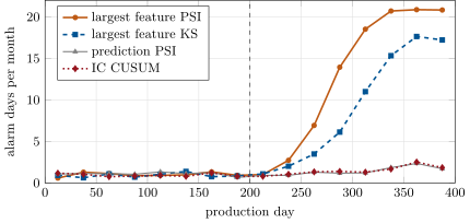
Method 27.4 (Designing a model’s monitors)

1. Monitor inputs, outputs and outcomes: each layer sees failures the others cannot.
2. Choose the false-page rate the team will actually answer, and calibrate every threshold to it on history or simulation without failures; do not copy thresholds from rules of thumb.
3. Count pages at the onset of an alarm, and distinguish a first page from a sustained alarm.
4. Measure each monitor’s delay on planted failures, and compare it with a blind monitor’s; a monitor that never beats that column is noise.
5. Accept that outcome monitors see only large losses quickly; cover small ones with scheduled revalidation.

27.4 Shadow, canary and champion–challenger rollouts

Definition 27.5 (Shadow deployment, champion–challenger)

In a shadow deployment a new model receives the production inputs and records its predictions, but its decisions are not executed; its outcomes are computed as if they had been. Champion–challenger is the discipline of keeping the production model (the champion) in place until a challenger, run beside it on the same data, has shown with a test chosen in advance that it is better.

A shadow run costs nothing but computation and gives a clean comparison, because champion and challenger see the same names on the same days. After the reversal, the CUSUM pages within days. A challenger is refitted on the 40 days that follow (its coefficient on the first feature is $-0.081$ on average over the runs, against the true $-0.08$) and runs in shadow from day 240. Its mean information coefficient is 0.105, the champion’s 0.003. The comparison uses Book 7’s always-valid sequential test (chapter 21) on the daily differences (Listing 27.5), which may be looked at every day without inflating its error rate; the standard error is estimated from the days seen, so the test gives no verdict for ten days, since on three days a small sample standard deviation makes any difference look certain. The challenger is promoted in all 20 runs, after a median of 10 shadow days and at most 19 (Figure 27.2). Without a failure, a challenger refitted on 40 ordinary days is promoted in 2 of 100 runs, within the test’s 5%.

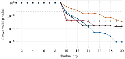
Shadow comparisons measure forecasts, not the market’s reaction to trading on them; a model whose orders move prices is compared in a canary deployment (Book 7, chapter 21), trading a small share of capital. The canary’s value is in what it limits. The chapter promotes a challenger with a sign error on its second feature, a bug a shadow run would have caught but suppose it did not: the CUSUM rolls it back after a median of 3 days (at most 18). The information coefficient given up, summed over those days and weighted by capital, is 0.26 IC-days when the challenger trades the whole book and 0.026 when it trades a tenth of it. The rollback itself is a registry action (Listing 27.6): the version that was in production before is promoted back, with the reason, into chapter 25’s audit trail.

27.5 Retrain, roll back, or retire

Each alarm calls for a different action, and the wrong one hides the failure. An input alarm with no fall in outcomes (the unit change) calls for fixing the data: retraining on volumes in lots would teach the model a new scale for one feature and bury the vendor’s error in its coefficients, until the vendor corrected it. An outcome alarm with calm inputs (the reversal) says the relation has changed: cut the model’s size or stop it (the kill switch of Book 11, chapter 27, for a model trading at speed), refit on data from after the change once there is enough, and promote through shadow and canary. A slow loss that no monitor sees is the case for scheduled retraining (chapter 12’s retraining schedule) and periodic revalidation of the model against a simple benchmark. A model is retired when its refitted challengers no longer beat a null: when the effect is gone, retraining only fits noise faster. Sculley and co-authors list “changes in the external world” among the debts of machine-learning systems, and Breck and co-authors make monitoring half of their rubric for a model’s production readiness. In the interviews of machine-learning engineers by Shankar and co-authors, false-positive alerts were the most commonly discussed pain point, and the alert fatigue that follows leads teams to silence alerts and miss real drops: the reason to count pages.

Method 27.6 (After an alarm)

1. Input or output alarm: check the data path first (units, schema, vendor changes); fix the data, not the model.
2. Outcome alarm with calm inputs: reduce or stop trading, refit on post-change data, and promote only through shadow and a canary.
3. A challenger is promoted by a sequential test chosen in advance, and rolled back by the performance alarm, both recorded in the registry.
4. Retrain on a schedule for the losses no monitor sees; retire the model when retraining no longer beats a null.

27.6 Tutorial: the Tuesday the model went quiet

27.7 Build: model monitoring

27.8 Exercises

Exercise 27.1 ★

For each of the three layers (inputs, outputs, outcomes), name one failure it sees that the other two do not, from the chapter’s three.

Solution

Solution of Exercise 27.1.

Inputs: the slow fade’s growing spread (seen by the feature index and Kolmogorov–Smirnov statistic, by nothing else). Outputs: the unit change as a rise of the share inside the trading threshold from 50% to 63%, which the inputs also see but which only the outputs translate into trading (a quarter fewer names traded). Outcomes: the reversal, invisible to inputs and outputs because neither the features nor the distribution of predictions change.

Exercise 27.2 ★

Why is the calibrated threshold on the largest feature index (0.115) above the credit-scoring rule of thumb of 0.10, and what would a threshold of 0.10 do?

Solution

Solution of Exercise 27.2.

With 200 names, each decile holds 20 names, and sampling noise alone gives each feature’s daily index a spread that puts the largest of five above 0.10 on more than one day in twenty. The rule of thumb was set for large credit portfolios and says nothing about error rates; a threshold of 0.10 here would page more often than once a month, and the team would learn to ignore it.

Exercise 27.3 ★

Why does a blind monitor, calibrated to one false page a month, still show a first alarm about two weeks after a failure?

Solution

Solution of Exercise 27.3.

Its false pages arrive at random, about one day in 21, so the wait for the first one after any date is geometric with a median of about 14 days (the table’s “none” column shows 10 to 17 for the five monitors). A first alarm means something only when it comes well before that.

Exercise 27.4 ★★

Check the chapter’s figure of about 150 days for the outcome monitor to see the unit change, from the information coefficients 0.103 and 0.087 and the daily standard deviation 0.071. How many days would a firm trading 2 000 names need?

Solution

Solution of Exercise 27.4.

$\Delta=0.103-0.087=0.017$ (unrounded 0.0168), $\sigma=0.071$, $z_{0.95}+z_{0.90}=1.645+1.282=2.927$: $n=(2.927\times0.071/0.0168)^2 \approx150$ days. The daily coefficient’s standard deviation shrinks roughly as one over the square root of the number of names; with 2 000 names it is about $0.071/\sqrt{10}=0.022$, and $n$ falls tenfold to about 15 days.

Exercise 27.5 ★★

Why does the shadow test give no verdict for ten days? What goes wrong without that rule?

Solution

Solution of Exercise 27.5.

The test’s standard error is estimated from the days seen so far. On three days the sample standard deviation of the differences can be tiny by chance, the estimated standard error with it, and a modest mean difference then looks overwhelming: with verdicts from the third day, one of the chapter’s runs shows a p-value of $1.3\times10^{-6}$ on that day. The test’s error guarantee assumes a known standard error; ten days are a burn-in that makes the estimate usable. Without a failure, verdicts from the third day promote 16 of 100 null challengers, against 2 with the burn-in.

Exercise 27.6 ★★

Find the flaw. “The PSI alarm went off after the vendor change, so we retrained the model on the new data and the alarm stopped.”

Solution

Solution of Exercise 27.6.

The alarm was right and the fix was wrong. The vendor’s change was a data error; retraining taught the model to multiply the feature in lots by a hundred times the coefficient, burying the error in the model. When the vendor corrects the feed, the retrained model is wrong by a factor of a hundred on that feature, and the alarm fires again. Fix the data (convert units at the boundary, add a schema or range check), keep the model.

Exercise 27.7 ★★★

Coding. Add the pooled monitor of the tutorial’s last step (the largest feature index over the last 20 days of samples), calibrate it to one page a month, and report its delays. Why do its false alarms come in spells?

Solution

Solution of Exercise 27.7.

ml_monitor.pooled: the pooled index’s threshold at one page a month is 0.0056, twenty times below the daily one, since 4 000 samples a feature carry much less noise than 200. Consecutive windows share 19 of their 20 days, so the statistic moves slowly and its false alarms come in spells, 3.7 alarm days per page on average. The first alarm does not beat a blind monitor (median 15.5 days for the fade, 18 without a failure), and the five-in-21 rule is tripped by a single false spell (median 20 days without a failure), so neither count means what it did. Measured by a month of continuous alarm, the pooled index sees the fade after a median of 22.5 days, against 120 for the daily index; but four of the 20 runs without failures also show a false month of continuous alarm. Pooling buys sensitivity to slow drifts with alarms that are fewer but longer, and harder to dismiss.

Exercise 27.8 ★★★

Design the monitors for a fade with no change of spread: the third feature’s effect falls to zero over 150 days and its distribution is unchanged. Which layer can see it, how fast, and what would you do instead?

Solution

Solution of Exercise 27.8.

No input or output monitor can see it: the features’ distribution is unchanged, and so, to first order, is that of the predictions. Only outcomes can, and the loss is gradual: the coefficient falls to 0.081 at the end of the fade, and the chapter’s formula needs about 80 days at that level, so the alarm would come months after the fade began, if at all at one false page a month. The practical answer is not a monitor but a schedule: refit or revalidate the model regularly (chapter 12), compare each feature’s recent contribution (its coefficient refitted on a rolling window) with the training one, and look at attribution of the realised IC by feature, which concentrates the evidence on the feature that fades.

27.9 Problem: The Tuesday the Model Went Quiet

Problem 27.1

Weekend problem — the Tuesday the model went quiet

The chapter’s simulated production run, three planted failures, five monitors.

Part I — The model and its monitors.

1. Describe the production model and the three failures.
2. What does each layer (inputs, outputs, outcomes) monitor, and when is each available?
3. Define the population stability index and give the calibrated thresholds.
4. Why count pages at the onset of an alarm?

Part II — Performance alarms.

5. How is the CUSUM on the information coefficient set up and calibrated?
6. How many days does an outcome monitor need to see each failure?
7. Why can outcomes not see the unit change?
8. What is the difference between a first alarm and a sustained alarm?

Part III — The delays.

9. Which monitors see the unit change, and when?
10. Which see the reversal?
11. What sees the slow fade, and through what?
12. What would have caught the fade without its change in spread?

Part IV — The verdict.

13. State the named result: each monitor’s detection delay for the three planted failures at one false alarm a month.
14. What happens in shadow after the reversal, and how often is a null challenger promoted?
15. What does a canary save when a faulty challenger is promoted?
16. What should the desk have done on the Tuesday?
17. When should a model be retrained, and when retired?
18. Who should be paged by each monitor?
19. What should the monitoring record in the registry?
20. In one sentence: what does a monitor need before it is worth having?

Solution

Solution of Problem 27.1.

Part I.

1. Two hundred names a day, five standardised features, next-day returns loading 0.08, $-0.06$ and 0.05 on the first three plus unit noise; a linear model fitted on 60 days runs for 400, trading the half of names with the largest forecasts. From day 200: the second feature a hundred times smaller; the first feature’s effect reversed; the third’s effect fading to zero over 150 days while its spread grows by half.
2. Inputs (feature distributions against the training reference; at once), outputs (distribution of predictions, share inside the trading threshold; at once), outcomes (realised information coefficient, P&L; after the horizon, and noisy).
3. $\sum_b(q_b-r_b)\ln(q_b/r_b)$ over the reference’s deciles; thresholds 0.115 (largest feature index), 0.115 (largest Kolmogorov–Smirnov statistic), 0.089 (index of the predictions), 0.07 (change in the share inside the threshold).
4. Because a person is paged once per episode, not once per day of it; calibrating on alarm days would make persistent statistics look noisier than they are.

Part II.

1. One-sided, on the daily coefficient’s shortfall below its expected 0.103, allowance $k=0.035$ (half the daily standard deviation of 0.071), threshold $h=0.11$ chosen on runs without failures to page once a month, reset after each page.
2. About $((z_{0.95}+z_{0.90})\sigma/\Delta)^2$: 4 days for the reversal, about 150 for the unit change, about 80 for the fade at its end.
3. The unit change removes one feature’s contribution from the forecast; the coefficient falls only from 0.103 to 0.087, a drop a quarter of a day’s noise.
4. A first alarm is the first page after the failure, which a blind monitor also produces within about two weeks; a sustained alarm is five alarm days in 21, which no monitor reaches without a failure.

Part III.

1. All four input and output monitors on the first day, sustained at once; the outcome monitor pages once after a median of 9.5 days and never insists.
2. Only the IC CUSUM: within two days in 13 of 20 runs, sustained at once.
3. Nothing sees its lost accuracy; the input monitors see its growing spread, sustained after a median of 42 days (feature index) and 60 (Kolmogorov–Smirnov).
4. Nothing in the table; a scheduled revalidation, or a monitor on each feature’s contribution to the realised coefficient.

Part IV.

1. The Tuesday the model went quiet. At one false page a month (medians over 20 runs; first alarm / sustained): unit change, every input and output monitor 0 / 0 days, IC CUSUM 9.5 days / never; reversal, input and output monitors no better than blind (10 to 17 days, never sustained), IC CUSUM 1 / 0 days; slow fade, feature index 12 / 42 days, Kolmogorov–Smirnov 8 / 60, prediction index, share inside and IC CUSUM never sustained.
2. A challenger refitted on 40 post-reversal days (information coefficient 0.105 against the champion’s 0.003) is promoted in all 20 runs after a median of 10 shadow days, at most 19; without a failure, 2 of 100 challengers are promoted.
3. A challenger with a sign error is rolled back by the CUSUM after a median of 3 days; the information coefficient given up is 0.26 IC-days at full size and 0.026 at a tenth.
4. Page the data owner on the share-inside and feature alarms, stop or shrink the model, find the unit change and fix the feed; not retrain.
5. Retrain after a confirmed change in the relation, once there is enough post-change data, and on a schedule; retire when refitted challengers no longer beat a null.
6. Input alarms: the data owner; output alarms: the desk and model owner; outcome alarms: the model owner and risk.
7. Every alarm, who acknowledged it, the action (data fix, size cut, rollback, promotion) with its reason, linked to the model version in the registry.
8. A false-alarm rate the team will answer and a measured delay on the failures it is for.

27.10 Interview questions

Interview question 27.1 ★ mle

What would you monitor for a model in production, and why at more than one layer?

Solution

Solution of Interview question 27.1.

Inputs (schema, freshness, feature distributions), outputs (prediction distribution, positions, turnover, share of trades) and outcomes (realised IC, P&L, mark-outs). Each layer sees failures the others miss: a unit change is loud in the inputs and faint in the outcomes; a regime change is silent in the inputs and loud in the outcomes.

What the interviewer is looking for: three layers and an example each.

Interview question 27.2 ★★ mle, researcher

What is the population stability index, and how would you choose its alarm threshold?

Solution

Solution of Interview question 27.2.

$\sum_b(q_b-r_b)\ln(q_b/r_b)$ over the reference’s bins. Choose the threshold for a false-alarm rate on data without failures (history or simulation), with the actual sample size and number of features monitored; the 0.10 and 0.25 rules of thumb ignore both.

What the interviewer is looking for: the formula and calibration to an error rate.

Interview question 27.3 ★★ researcher

Your model’s daily IC is 0.10 with a standard deviation of 0.07. How long before you could tell it had fallen to 0.08?

Solution

Solution of Interview question 27.3.

$\Delta=0.02$, $\sigma=0.07$: $((1.645+1.282)\times0.07/0.02)^2\approx105$ days, five months, for a one-sided 5% test with 90% power; more names shorten it, as $\sigma$ falls roughly with the square root of their number.

What the interviewer is looking for: the sample-size arithmetic and its dependence on breadth.

Interview question 27.4 ★★ mle

Explain shadow deployment, canary and champion–challenger. When is each the right tool?

Solution

Solution of Interview question 27.4.

Shadow: the new model sees live inputs and its decisions are scored but not executed; right for comparing forecasts at no risk. Canary: it trades a small share of capital; right when its trading changes outcomes (impact, fills). Champion–challenger: the discipline around both, keeping the incumbent until the challenger wins a test chosen in advance.

What the interviewer is looking for: what each measures and risks.

Interview question 27.5 ★★ mle, developer

Your input drift alarm fires. Do you retrain?

Solution

Solution of Interview question 27.5.

Not first. Check whether the drift is a data error (units, schema, a vendor change) or a real change in the population; fix data errors at the source. If the population really changed, check the outcomes: a model can be robust to covariate shift; retrain when the outcomes or a revalidation say it is not, and promote through shadow.

What the interviewer is looking for: data path first, outcomes before retraining.

Interview question 27.6 ★★★ mle

Your monitors page the team twenty times a week and nobody looks any more. What do you change?

Solution

Solution of Interview question 27.6.

Measure each monitor’s false-page rate and its delay on the failures it exists for; drop monitors that never beat a blind one; recalibrate the rest to a rate the team will answer (count pages at onset); route each alarm to its owner; group related alarms; and cover slow losses with scheduled reviews instead of pages.

What the interviewer is looking for: calibration to a rate, measured value per monitor, routing.