Machine Learning for Markets · Machine learning

21Interpretability and Model Governance

A risk committee asks why the model cut its position in a stock by half on Tuesday. The researcher’s answer, that the gradient-boosted model’s output fell, is true and useless. The committee wants to know which inputs moved, whether the model’s response to them makes sense, whether it would have said the same last month, and who checked. This chapter is about answering those questions honestly: explanations that are right about the model even when the features are correlated, explanations that survive a retrain, and the documents (a model card, a validation report) through which a learned model enters the firm’s model risk management (Book 6, chapter 26). Two measurements anchor it. With two features correlated at 0.99, partial dependence misstates a feature’s effect by twice as much as accumulated local effects. And on a problem with a realistic signal-to-noise ratio, the top five features by SHAP value are never the same five across ten retrains.

21.1 What an explanation is for

Definition 21.1 (Interpretability)

Interpretability is the degree to which a person can understand why a model produces its outputs: globally (how the prediction depends on each input across the data) or locally (why this prediction, for this input). An explanation is itself a model of the model, and has an accuracy of its own.

Explanations serve different readers. A researcher uses them to debug: a feature that matters and should not is a leak (chapter 3). A risk manager uses them to check that the model’s responses have the right sign and size, and that it will not do something absurd in a market it has not seen. A committee or a regulator uses them to decide whether the firm understands what it runs. Rudin (2019) argued that for high-stakes decisions an interpretable model should be preferred to an explained black box; in trading, where the models are often small and the signal weak, that is a live option (chapter 4’s baselines), and a learned model should earn its complexity against it. The chapter’s model is a gradient-boosted regression (chapter 5) fitted to $y = x_1 + x_2^2 + 2x_3x_4 + \varepsilon$ on 6 000 observations, where $x_2$ is, in two variants, a noisy copy of $x_1$ (correlations 0.92 and 0.99).

21.2 Global explanations: partial dependence and accumulated local effects

Definition 21.2 (Partial dependence, individual conditional expectation, accumulated local effects)

The partial dependence of a model $f$ on feature $j$ is $\mathrm{PD}_j(v) = n^{-1}\sum_i f(v, x_{i,-j})$ : the average prediction with feature $j$ set to $v$ for every observation (Friedman, 2001). The individual conditional expectation (ICE) curves are the terms of that average, one curve per observation (Goldstein and co-authors, 2015). Accumulated local effects (ALE) average, within narrow intervals of feature $j$ , the change in prediction when $j$ moves across the interval for the observations that lie in it, and accumulate those changes (Apley and Zhu, 2020).

Partial dependence asks what the model predicts for combinations of features that may never occur: with $x_2$ nearly equal to $x_1$ , setting $x_1 = -0.9$ for an observation with $x_2 = 0.9$ asks the model about a point where it has no data, and a tree ensemble answers with whatever its last split there says. ALE only moves each observation across a short interval around its own value (Listing 21.1). Table 21.1 measures both against the true effect of $x_1$ , a straight line of slope 1, and Figure 21.1 shows them at correlation 0.99.

	correlation of $x_1$ and $x_2$
root mean square error against the true effect of $x_1$	0	0.92	0.99
partial dependence	0.027	0.134	0.229
accumulated local effects	0.028	0.044	0.110

Table 21.1. Error of two global explanations of the same fitted model, evaluated at the data’s values of

x_1

(the true effect ranges over 2). Data: ml_explain.effects.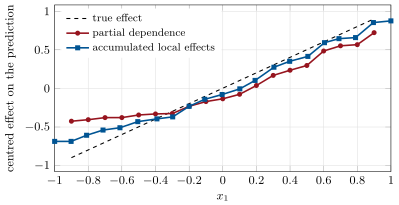

The effect of x_1 on a gradient-boosted model when x_2 is a copy of x_1 with correlation 0.99. Data: ml_explain.curves. — **Figure 21.1.** The effect of $x_1$ on a gradient-boosted model when $x_2$ is a copy of $x_1$ with correlation 0.99. Data: `ml_explain.curves`.

With independent features the two agree. As the correlation rises, partial dependence absorbs part of $x_2$ ’s quadratic effect into $x_1$ and its error grows five- and eightfold; ALE’s grows too, because a model trained on nearly identical features cannot itself say which one carries which effect, but it stays at half of partial dependence’s. No explanation can separate effects that the data do not separate; ALE at least does not add errors from places the data never visited.

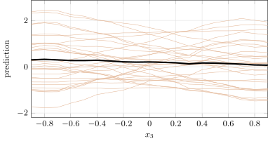
ICE curves show what an average hides. The partial dependence of $x_3$ is flat (slope 0.009): its effect is entirely its interaction with $x_4$ . The ICE curves of 30 observations (Figure 21.2) fan out with slopes whose standard deviation is 0.91 and whose correlation with the observation’s $x_4$ is 0.98: the model has learned the interaction, and the average of its responses has erased it.

ICE curves of x_3 for 30 observations (thin) and their average (thick), for the model with independent features. Data: ml_explain.ice_x3. — **Figure 21.2.** ICE curves of $x_3$ for 30 observations (thin) and their average (thick), for the model with independent features. Data: `ml_explain.ice_x3`.

Definition 21.3 (Global surrogate)

A global surrogate is an interpretable model (a shallow tree, a linear model) fitted to a complex model’s predictions; its fidelity, the share of the predictions’ variance it reproduces, says how much of the model it explains.

A depth-three tree fitted to the model’s predictions splits only on $x_1$ and $x_2$ and reproduces 48% of their variance: it explains the additive half of the model and none of the interaction. A surrogate is an honest explanation only with its fidelity printed next to it.

21.3 Local explanations and their stability

Definition 21.4 (Counterfactual explanation)

A counterfactual explanation of a prediction is the smallest change of the inputs that would have changed the decision, for example the value of one feature at which the forecast changes sign (Wachter, Mittelstadt and Russell, 2017).

Local explanations answer the committee’s question about Tuesday. SHAP values (chapter 6) split one prediction among the features; a counterfactual says what would have had to be different. For one observation of the chapter’s model, whose prediction is 0.82 with $x_1 = 0.46$ , the forecast turns negative only if $x_1$ falls to $-0.44$ : most of this prediction comes from the interaction, and $x_1$ alone would need a large move to reverse it.

An explanation that changes with every retrain explains the training run, not the market. Figure 21.2 and the table above come from one fit; the chapter also retrains a model ten times on bootstrap resamples of a problem with three strong features (coefficients 1, 0.7, 0.5), five weak ones (0.2 each) and twelve with no effect, and ranks the features by mean absolute SHAP value each time (Listing 21.2). When the features explain 66% of the variance, the top five features are the same set in 22% of retrains, and the first retrain’s top five keep their order with a mean Kendall correlation of 0.89: the three strong features are always first, and which two weak features complete the list is a coin toss among five equals. When they explain 5%, closer to a return forecast, the top five are never the same set and the Kendall correlation falls to 0.78; in some retrains a null feature enters the top five. A report that names “the model’s five most important features” from one fit is reporting noise in its last two places.

21.4 Documentation: the model card

Definition 21.5 (Model card)

A model card is a short document that travels with a model and states its purpose, training data, evaluation, performance by relevant slices, behaviour, limitations and approvals (Mitchell and co-authors, 2019); in a firm it is the learned model’s entry in the model inventory (Book 6, chapter 26).

The card is generated, not written: its fields are filled from the training run and the validation report, and the generator refuses to call a card complete with fields missing. The chapter’s card for its demonstration model lists fifteen fields and reports two missing, monitoring and approvals, which is exactly the state of a model that has been built and validated but not deployed. Its limitations field records the one fact a user must know: where $x_1$ and $x_2$ are correlated, read ALE, not partial dependence.

As of September 2026 — Model risk rules and learned models

The United States’ model risk guidance was revised on 17 April 2026 (SR 26-2, superseding SR 11-7); Book 6 (chapter 26) describes both. The Prudential Regulation Authority’s supervisory statement SS1/23, Model risk management principles for banks, published on 17 May 2023, sets five principles and applies them to all models used to inform business decisions, “regardless of technology”, including “the use of artificial intelligence in modelling techniques such as machine learning to the extent that it applies to the use of models more generally”; its current version took effect on 23 April 2026, after the PRA’s April 2026 low-impact amendments.

21.5 Validating a learned model

Validation of a learned model asks the questions of Book 6 (conceptual soundness, outcomes analysis, benchmarking, effective challenge) plus a few that learned models make pressing: leakage, stability across retrains, and parity between the model that was validated and the one that runs. Table 21.2 is the chapter’s checklist for its demonstration model, filled where the evidence exists and marked “not run” where it does not; the numeric items run through Book 6’s firm.modelval.

item	result	evidence
out-of-sample performance	pass	$R^2$ 0.860 on 2 000 new observations
challenger comparison	pass	ridge regression $R^2$ 0.349 on the same observations
implementation parity	pass	the exported trees (chapter 5) reproduce the model exactly on 200 rows
outcomes analysis	pass	27 of 250 outcomes outside the 90% interval (25 expected), binomial tail 0.37
conceptual soundness, leakage, stability, explanations, monitoring	not run	to be filled by the validator

Table 21.2. The validation checklist of the chapter’s model. Data: ml_explain.validation.

Method 21.6 (Explaining and governing a learned model)

Explain effects with ALE where features are correlated, show ICE curves where interactions are suspected, and print a surrogate’s fidelity with the surrogate.
Report feature rankings from several retrains, with their stability; name only the features that are stable.
Answer questions about single decisions with SHAP values and counterfactuals computed on the deployed model.
Generate the model card from the training and validation records; register it in the model inventory; let the validator fill the checklist, and do not deploy with items not run.

21.6 Tutorial: explain it to the risk committee

Goal. Explain a boosted model with PD, ICE, ALE and a surrogate; measure the stability of its SHAP rankings; generate its card and checklist. End state: Tables 21.1 and 21.2, Figures 21.1 and 21.2.

Accumulated local effects.

def ale(predict, X, j, bins=20):
    """First-order accumulated local effect: within each quantile bin of feature j, the mean change in prediction when
    j moves from the bin's lower to its upper edge, the other features kept at their observed values; accumulated
    over bins and centred to mean zero over the data."""
    x = X[:, j]
    edges = np.unique(np.quantile(x, np.linspace(0, 1, bins + 1)))
    idx = np.clip(np.searchsorted(edges, x, side="right") - 1, 0, len(edges) - 2)
    local = np.zeros(len(edges) - 1)
    counts = np.zeros(len(edges) - 1)
    for b in range(len(edges) - 1):
        rows = idx == b
        if not rows.any():
            continue
        lo, hi = X[rows].copy(), X[rows].copy()
        lo[:, j], hi[:, j] = edges[b], edges[b + 1]
        local[b] = float(np.mean(predict(hi) - predict(lo)))
        counts[b] = rows.sum()
    acc = np.r_[0.0, np.cumsum(local)]
    mid = 0.5 * (acc[:-1] + acc[1:])
    return edges, acc - float((mid * counts).sum() / counts.sum())

Listing 21.1. First-order ALE with quantile bins. code/firm/modelcard/firm_modelcard.py

Stability of rankings across retrains.

def rank_stability(rankings, top=5):
    """rankings: list of feature-index arrays, most important first. The share of retrains whose top-`top` set equals
    the first retrain's, and the mean Kendall tau between the first retrain's top features' ranks and each other's."""
    ref = list(rankings[0][:top])
    same = [set(r[:top]) == set(ref) for r in rankings[1:]]
    taus = []
    for r in rankings[1:]:
        pos = {f: i for i, f in enumerate(r)}
        taus.append(_kendall(list(range(top)), [pos[f] for f in ref]))
    return float(np.mean(same)), float(np.mean(taus))

Listing 21.2. Top-set agreement and Kendall correlation across retrains. code/firm/modelcard/firm_modelcard.py

Run ml_explain.effects(), ice_x3(), surrogate(), stability(1.0), stability(6.0), validation(), card().render() and fig_explain.py.

What to change next. Add second-order ALE for the pair $(x_3, x_4)$ ; replace bootstrap retrains by retrains on successive years; add a leakage canary (chapter 3) to the checklist.

21.7 Build: explanations and model cards

Purpose. Explanations whose accuracy and stability are measured, and a learned model documented and validated like any other model.

Interface. partial_dependence, ice, ale, global_surrogate, counterfactual, rank_stability; ModelCard with render and missing; benchmark_check, outcome_check, validation_checklist (on firm.modelval).

Rules. No explanation without its accuracy or fidelity; no ranking without its stability; no card with missing fields marked complete; checklist items without evidence are “not run”.

Acceptance tests. code/firm/modelcard/tests/: PD and ALE recover a known additive function; ALE is right and PD wrong on a correlated pair with an off-manifold trap; ICE slopes recover an interaction; a surrogate of a tree is perfect; counterfactuals cross the threshold; rank stability is 1 for identical rankings; the card lists its missing fields.

Stretch. Second-order ALE; SHAP interaction values; cards in the experiment tracker (chapter 25).

Sources and further reading

J. H. Friedman, “Greedy function approximation: a gradient boosting machine”, Annals of Statistics 29(5), 2001.
A. Goldstein, A. Kapelner, J. Bleich and E. Pitkin, “Peeking inside the black box: visualizing statistical learning with plots of individual conditional expectation”, Journal of Computational and Graphical Statistics 24(1), 2015.
D. W. Apley and J. Zhu, “Visualizing the effects of predictor variables in black box supervised learning models”, Journal of the Royal Statistical Society B 82(4), 2020.
M. Mitchell and co-authors, “Model cards for model reporting”, FAT*, 2019.
S. Wachter, B. Mittelstadt and C. Russell, “Counterfactual explanations without opening the black box: automated decisions and the GDPR”, SSRN 3063289, 2017.
C. Rudin, “Stop explaining black box machine learning models for high stakes decisions and use interpretable models instead”, Nature Machine Intelligence 1, 2019.
Prudential Regulation Authority, SS1/23, Model risk management principles for banks, 2023 (current version 2026).

21.8 Exercises

Exercise 21.1 ★

For $f(x_1, x_2) = x_1 + x_2^2$ with $x_1$ and $x_2$ independent and uniform on $[-1, 1]$ , write the partial dependence on $x_1$ . What changes if $x_2 = x_1$ exactly and the model is $f$ itself?

Solution

Solution of Exercise 21.1.

$\mathrm{PD}(v) = v + \E[x_2^2] = v + 1/3$ : the true effect plus a constant. If $x_2 = x_1$ and the model is $f$ itself, partial dependence still averages $x_2^2$ over the marginal of $x_2$ and returns $v + 1/3$ , while along the data the prediction is $v + v^2$ : partial dependence describes the formula, not what the model does on the data, and attributes none of the curvature to the only variable that moves.

Exercise 21.2 ★

With 250 outcomes and a 90% interval, how many exceptions are expected? Is 27 alarming?

Solution

Solution of Exercise 21.2.

$0.1\times250 = 25$ expected. The probability of 27 or more is 0.37: not alarming.

Exercise 21.3 ★

A global surrogate has fidelity 0.48. What can and cannot be said from it?

Solution

Solution of Exercise 21.3.

The tree’s rules describe the part of the model’s behaviour it reproduces, less than half of the variance here; nothing may be concluded about the rest, which here is the whole interaction. A surrogate’s rules are an explanation only where its fidelity is high, and should be checked on the slices that matter.

Exercise 21.4 ★★

Why is the partial dependence of $x_3$ flat although $x_3$ matters?

Solution

Solution of Exercise 21.4.

Its effect is $2x_3x_4$ with $x_4$ symmetric around zero: for every observation where raising $x_3$ raises the prediction there is one where it lowers it, and the average slope is zero. The ICE curves’ slopes follow $x_4$ .

Exercise 21.5 ★★

Why do the fourth and fifth places of the SHAP ranking change across retrains even with a strong signal?

Solution

Solution of Exercise 21.5.

The five weak features have equal true effects; their estimated importances differ by sampling noise, which reorders them in every resample. Only differences of importance larger than that noise are stable.

Exercise 21.6 ★★

Find the flaw. “The model’s SHAP values show that the earnings-revision feature drives 40% of the forecast, so the model is a revisions model and the committee can think of it that way.”

Solution

Solution of Exercise 21.6.

A share of SHAP attribution from one fit, with correlated features and no stability check, does not say the model is a revisions model: correlated features share credit arbitrarily, the share may change at the next retrain, and attribution is not causation. Show ALE and ICE for the feature, the attribution across retrains, and the performance of the model without it.

Exercise 21.7 ★★★

Coding. Rerun the stability experiment at the high signal level with ten retrains on disjoint tenths of the data (400 observations each) instead of bootstrap resamples of all 4 000. Does stability rise or fall, and why?

Solution

Solution of Exercise 21.7.

It appears to rise to perfection: the top five are features 0 to 4 in every retrain and the Kendall correlation is 1. The explanation is that nothing was learned: with 400 observations, bagging at 70% and the firm’s minimum of 200 observations per leaf, no tree can split, every SHAP value is zero, and the ranking falls back to the column order. A stability score must be read with the importances it ranks.

Exercise 21.8 ★★★

Show that for an additive model $f = \sum_jf_j(x_j)$ the ALE of feature $j$ equals $f_j$ up to a constant whatever the dependence between the features, and that partial dependence does too. Where, then, does partial dependence go wrong?

Solution

Solution of Exercise 21.8.

ALE of $j$ accumulates $\E[f(z_{k}, x_{-j}) - f(z_{k-1}, x_{-j})\mid x_j\in(z_{k-1}, z_k]]$ ; for an additive $f$ the other components cancel in each difference, leaving $f_j(z_k) - f_j(z_{k-1})$ , and the sum telescopes to $f_j$ plus a constant. Partial dependence is $f_j(v) + \sum_{k\ne j}\E f_k(x_k)$ , also $f_j$ plus a constant. Both are right for the true additive function; partial dependence goes wrong for a fitted model, which is only constrained where the data are and may not be additive off the data’s support, where partial dependence evaluates it.

21.9 Problem: Explain It to the Risk Committee

Problem 21.1

Weekend problem — an explanation has an error bar

The chapter’s model, retrains, card and checklist.

Part I — Global effects.

What are the errors of PD and ALE at each correlation?
Why does ALE’s error grow too?
What do the ICE curves of $x_3$ show that PD does not?
What does the surrogate explain, and what does it miss?

Part II — Local and stable.

What does the counterfactual say about the example’s prediction?
How stable is the top five at each signal level?
What should a report on feature importance contain?
How would you answer the committee’s question about Tuesday?

Part III — Governance.

What does the model card contain, and what is missing?
Which checklist items pass, on what evidence?
Why is implementation parity on the list?
What does the dated box say about how supervisors treat learned models?

Part IV — The verdict.

State the named result: partial dependence’s error against the true effect under correlated features compared with ALE’s, and the rank stability of the top five SHAP features across ten retrains.
Would you replace the boosted model by an interpretable one here?
Which tier (Book 6) would you give a learned alpha model, and why?
What does effective challenge look like for a learned model?
What must be re-validated after a retrain?
How do you explain a model whose inputs are embeddings (chapter 10)?
What should never be in a model card?
In one sentence: what is an explanation?

Solution

Solution of Problem 21.1.

Part I.

At correlations 0, 0.92 and 0.99: PD 0.027, 0.134, 0.229; ALE 0.028, 0.044, 0.110.
The fitted model itself cannot separate nearly identical features; ALE explains the model, which mixes their effects.
Slopes spread with standard deviation 0.91 and correlation 0.98 with $x_4$ : the interaction.
The additive part in $x_1$ and $x_2$ (fidelity 0.48); none of the interaction.

Part II.

The prediction (0.82) comes mostly from the interaction; $x_1$ would have to fall from 0.46 to $-0.44$ to reverse it.
At $R^2$ 0.66: the same set in 22% of retrains, Kendall 0.89; at $R^2$ 0.05: never, Kendall 0.78, with null features sometimes in the top five.
Importances from several retrains, their spread, the features stable at the top, and a warning on correlated groups.
With the deployed model’s SHAP values for that stock on Monday and Tuesday, the inputs that changed, a counterfactual, and the ALE of those inputs showing that the response is sensible.

Part III.

Fifteen fields from name to approvals; monitoring and approvals are missing.
Out-of-sample performance ( $R^2$ 0.860), the challenger (ridge 0.349), implementation parity (exact on 200 rows) and outcomes (27 of 250, tail 0.37).
The model that runs must be the model that was validated; exports, compilers (chapter 26) and retrains break that silently.
That supervisors treat learned models as models, under the same principles, whatever the technology.

Part IV.

Explain it to the risk committee. Partial dependence’s error against the true effect is 0.134 and 0.229 at correlations 0.92 and 0.99, against ALE’s 0.044 and 0.110; the top five SHAP features are the same set in 22% of ten retrains at $R^2$ 0.66 (Kendall 0.89) and in none at $R^2$ 0.05 (Kendall 0.78).
Not here, where the interaction carries half the signal and the challenger loses it; yes where a linear model is within noise of the boosted one.
A high tier if it drives positions at size: material, complex and uncertain.
An independent team rebuilding the model from the card, a challenger, stress inputs outside the training range, and explanations checked against economic sense.
Performance, stability, explanations and parity; the card’s version and data fields.
At the level of the features that feed the embedding, or with probes that relate embedding directions to known features.
Secrets (credentials, client data) and claims without evidence.
A model of the model, with an error of its own.

21.10 Interview questions

Interview question 21.1 ★ researcher, mle

What is the difference between partial dependence and ALE, and when does it matter?

Solution

Solution of Interview question 21.1.

Partial dependence averages predictions with the feature forced to each value for every observation, visiting combinations absent from the data; ALE averages local differences within intervals, for observations actually there. With correlated features partial dependence can be badly wrong; ALE stays on the data.

What the interviewer is looking for: the two definitions and the off-manifold problem.

Interview question 21.2 ★★ researcher

How stable are SHAP-based feature rankings, and how would you measure it?

Solution

Solution of Interview question 21.2.

Often unstable below the top few features, especially with weak signals and correlated features. Measure by retraining on resamples or successive periods and reporting top-set agreement and rank correlations, alongside the importances themselves.

What the interviewer is looking for: instability of the tail of the ranking and a measurement protocol.

Interview question 21.3 ★★ mle

What goes into a model card for a trading model?

Solution

Solution of Interview question 21.3.

Purpose and use, target and horizon, data and period, features, training procedure, validation results with a challenger, performance by regime, explanations, limitations, monitoring, owners and approvals, version.

What the interviewer is looking for: purpose, data, evaluation, limitations and ownership.

Interview question 21.4 ★★ researcher, trader

A portfolio manager asks why the model sold a stock. What do you show?

Solution

Solution of Interview question 21.4.

The forecast’s change and the inputs that drove it (SHAP on the deployed model), whether the response is sensible (ALE/ICE), what would have reversed it, and how the position rule turned the forecast into the trade.

What the interviewer is looking for: local attribution, sanity of the response, and the link to the position.

Interview question 21.5 ★★ mle, researcher

How would you validate a gradient-boosted model before production?

Solution

Solution of Interview question 21.5.

Out-of-time performance against a simple challenger, leakage checks, stability across retrains, explanations checked for sign and size, implementation parity of the exported model, outcomes analysis, a model card, and monitoring before go-live.

What the interviewer is looking for: challenger, leakage, stability, parity and monitoring.

Interview question 21.6 ★★★ researcher

When would you prefer an interpretable model to an explained black box in trading?

Solution

Solution of Interview question 21.6.

When the interpretable model is within noise of the black box, when decisions must be justified case by case, and when the cost of an unexplained failure is high; the weak signals of trading often make the first condition true.

What the interviewer is looking for: performance parity and the cost of opacity.

Terms defined in this chapter

See all 2333 terms in the glossary