Machine Learning for Markets · Machine learning

17Reinforcement Learning Foundations

An agent learns to sell a block of shares by trial and error in a simulator and beats the desk’s schedule by 0.9 basis points per lot. In the market the simulator was built from, it loses 0.6 basis points to the same schedule. The simulator had one wrong detail, liquidity that alternated every period instead of persisting, and the agent had learned to exploit it: it waited out every thin period for the deep one that the simulator always delivered next. Reinforcement learning is optimal control learned from experience instead of solved from a model (Book 4, chapter 9); what it learns is the environment it was trained in. This chapter works on a problem small enough to solve exactly, so that every learner can be measured against the truth: the value methods, the policy methods, bandits, the evaluation of a new policy from old logs, and the gap between a simulator and a market. Chapter 18 applies them to execution and market making.

17.1 Markov decision processes and the Bellman equations

Definition 17.1 (Reinforcement learning, Markov decision process, policy, reward, cumulative reward)

Reinforcement learning learns how to act from the consequences of actions. A Markov decision process (MDP) is a set of states $x$ , actions $u$ , transition probabilities $\P(x_{t+1}\mid x_t, u_t)$ and a reward $g_{t+1}$ received after each action; the cumulative reward from time $t$ is $G_t = \sum_{k\ge0}\gamma^kg_{t+k+1}$ , with a discount $\gamma\in(0,1]$ ( $\gamma = 1$ on the finite horizons of this chapter). A policy $\pi(u\mid x)$ gives the probability of each action in each state.

Definition 17.2 (Action-value function, Bellman equation)

The action-value function of a policy is $Q^\pi(x, u) = \E_\pi[G_t\mid x_t = x, u_t = u]$ , the expected cumulative reward of taking $u$ in $x$ and following $\pi$ afterwards; the value function of Book 4 is $V^\pi(x) = \sum_u\pi(u\mid x)Q^\pi(x, u)$ . The Bellman equation is the recursion $Q^\pi(x, u) = \E[g_{t+1} + \gamma V^\pi(x_{t+1})\mid x, u]$ ; for the optimal policy, $Q^*(x, u) = \E[g_{t+1} + \gamma\max_{u'}Q^*(x_{t+1}, u')\mid x, u]$ .

The chapter’s problem is to sell 10 lots in 10 periods. The state is the period, the lots left and the liquidity, deep or thin, which persists from one period to the next with probability 0.8. Selling $u$ lots costs $\eta u^2$ basis points of temporary impact, with $\eta = 0.5$ when liquidity is deep and 2 when it is thin; holding $q$ lots after a sale costs $0.2 q^2$ for the risk of the price moving; whatever is left is sold in the last period. The reward is minus the cost. With 242 states, backward induction on the Bellman equation (Listing 17.1) solves it exactly: the optimal policy costs 2.59 basis points per lot (risk included), selling 5 lots at once if liquidity is deep and 2 if it is thin. The desk’s schedule, the best one that ignores liquidity, costs 3.27; selling one lot a period costs 6.76, because of the risk of holding the block.

17.2 Value methods: temporal differences and Q-learning

Definition 17.3 (Temporal-difference learning, Q-learning)

Temporal-difference learning updates an estimate of a value towards a target built from the next reward and the current estimate of the next state’s value, $V(x_t)\leftarrow V(x_t) + \eta_\alpha\delta_t$ with $\delta_t = g_{t+1} + \gamma V(x_{t+1}) - V(x_t)$ , without waiting for the end of the episode. Q-learning applies it to action values with the target $g_{t+1} + \gamma\max_{u'}Q(x_{t+1}, u')$ , which learns the optimal policy’s values while acting otherwise (Watkins and Dayan, 1992); SARSA uses the action actually taken next, and learns the values of the policy it follows.

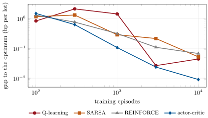
Listing 17.2 is tabular Q-learning with a step size of 0.1 and $\varepsilon$ -greedy exploration (a random action one time in ten). Figure 17.1 shows the value gap of the learned policy, measured exactly, against the number of episodes, averaged over three seeds. After 1 000 episodes Q-learning’s greedy policy is still 1.41 basis points per lot from the optimum; after 10 000 it is 0.044 away. SARSA, which learns the value of its own exploring policy, is safer early (0.28 at 1 000 episodes) and ends at 0.051.

17.3 Policy methods: gradients and actor-critic

Definition 17.4 (Policy gradient, actor–critic method)

A policy gradient method adjusts the parameters $\theta$ of a stochastic policy in the direction $\E[G_t\nabla_\theta\log\pi_\theta(u_t\mid x_t)]$ , the gradient of expected cumulative reward (REINFORCE; Williams, 1992); a baseline subtracted from $G_t$ lowers the variance without biasing it. An actor–critic method replaces $G_t$ by the temporal-difference error of a learned value function (the critic), so that the policy (the actor) learns at every step.

REINFORCE with a softmax policy and a baseline per state learns slowly and noisily: 0.31 basis points from the optimum after 1 000 episodes, 0.067 after 10 000, and with a larger step size it settled on a worse policy that it never left. The actor-critic of Listing 17.3 learns fastest here (0.11 at 1 000 episodes, 0.009 at 10 000). Policy methods matter when actions are continuous or many, where a maximum over actions is expensive, and when a stochastic policy is itself the goal; deep versions replace the tables by networks (Mnih and co-authors, 2015, for value methods).

Value gap to the dynamic-programming optimum of the policy learned after a number of episodes (the greedy policy for Q-learning and SARSA, the softmax policy for the others), mean of three seeds. Data: ml_rl.learning_curves. — **Figure 17.1.** Value gap to the dynamic-programming optimum of the policy learned after a number of episodes (the greedy policy for Q-learning and SARSA, the softmax policy for the others), mean of three seeds. Data: `ml_rl.learning_curves`.

17.4 Bandits and exploration

Definition 17.5 (Exploration–exploitation trade-off, multi-armed bandit, contextual bandit)

The exploration–exploitation trade-off is the choice between the action that looks best now and an action that teaches more. A multi-armed bandit is the MDP with one state: each round an arm is chosen and its reward drawn; the loss against always playing the best arm is the regret. A contextual bandit observes a context (the order, the market) before choosing, and learns a reward model per arm; its actions do not change future contexts.

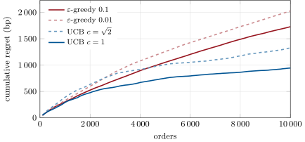
Five execution algorithms save 0, 0.5, 1.0, 1.2 and 1.5 basis points per order on average, with 5 basis points of noise per order. Over 10 000 orders (Figure 17.2), $\varepsilon$ -greedy with $\varepsilon = 0.1$ loses 1 727 basis points of cumulative saving against always using the best algorithm, and uses it for 78% of the last thousand orders; with $\varepsilon = 0.01$ it explores too little and locks on the wrong algorithm in some runs (2 026, 65%). The upper confidence bound rule, choosing the arm with the highest mean plus $c$ noise standard deviations times $\sqrt{\ln t/n_a}$ (Auer, Cesa-Bianchi and Fischer, 2002), loses 1 325 with $c = \sqrt2$ and 944 with $c = 1$ (83% and 87%): it explores the arms it is unsure of, not at random. Most of the loss is inevitable: an arm 0.3 basis points worse than the best, under 5 of noise, needs about two thousand orders on each to be told apart at two standard errors.

Cumulative regret of four exploration rules choosing among five execution algorithms, mean of 20 runs. Data: ml_rl.bandits. — **Figure 17.2.** Cumulative regret of four exploration rules choosing among five execution algorithms, mean of 20 runs. Data: `ml_rl.bandits`.

17.5 Off-policy evaluation and the simulator problem

Definition 17.6 (Off-policy evaluation, doubly robust estimator)

Off-policy evaluation estimates the value of a target policy from episodes generated by another, the behaviour policy, typically by reweighting each episode by the ratio of the two policies’ probabilities of the actions taken (importance sampling, Book 4, chapter 26). The doubly robust estimator adds to a model’s estimate of the target’s value the importance-weighted errors of the model on the logged rewards; it is unbiased if either the probabilities or the model are right, and has lower variance than importance sampling when the model is close (Dudík, Langford and Li, 2011).

A desk rarely gets to try a new policy on real orders before it knows its value. Here the desk’s logs come from its own schedule with random deviations 30% of the time (cost 3.80); the target is the optimal policy with deviations 10% of the time, so that every action it can take was sometimes logged (true cost 2.77). Table 17.1 compares the estimators on 100 sets of 300 logged episodes; the model given to the doubly robust estimator has the thin-liquidity impact half too high and liquidity too changeable.

estimator	bias	standard deviation	root mean square error
per-decision importance sampling	0.20	1.75	1.76
weighted importance sampling	0.49	0.63	0.80
model alone	0.30	0	0.30
doubly robust	$-0.03$	0.29	0.29

Table 17.1. Estimates of the target policy’s cost (true value 2.77 bp per lot) from 300 logged episodes of the desk’s behaviour policy, over 100 repetitions (bp per lot). Data: ml_rl.off_policy.

Importance sampling is unbiased and useless alone: products of ten probability ratios make a few episodes dominate. Weighting them to sum to one trades variance for bias. The model alone is precise and wrong; the doubly robust estimator keeps the model’s precision and removes most of its bias (Listing 17.4).

Definition 17.7 (Sim-to-real gap)

The sim-to-real gap is the difference between a policy’s performance in the simulator it was trained in and in the real environment. It is largest for policies that exploit what the simulator gets wrong, which is what an optimiser does with any error that pays.

The hook’s agent is Q-learning trained for 10 000 episodes in a simulator identical to the market except that liquidity alternates every period, as it did in a calendar pattern in the data the simulator was calibrated on (Book 7, chapter 19). In the simulator it costs 2.77 basis points per lot against the desk’s 3.66. In the market it costs 3.83 against the desk’s 3.27 and the optimum’s 2.59: waiting for deep liquidity that does not come, it carries its risk longer and sells into thin markets at the end. The desk’s schedule, which assumed nothing about liquidity, lost nothing when the assumption was wrong.

Method 17.8 (Before trusting a learned policy)

Solve the smallest version of the problem exactly and check that the learner finds it.
Estimate the new policy’s value from real logs by off-policy evaluation, with a doubly robust estimator and the behaviour policy’s logged probabilities; log them for every decision.
Evaluate the policy in simulators that differ from the training one in the assumptions it might exploit (persistence, impact, fills), and prefer policies whose value is stable across them.
Compare with the simplest schedule that assumes least, and deploy with limits (chapter 18).

17.6 Tutorial: learning to sell

Goal. Solve the liquidation MDP exactly, learn it four ways, run the bandits, evaluate a policy from logs and train in a wrong simulator. End state: Figures 17.1 and 17.2, Table 17.1.

Backward induction.

    def solve(self):
        """Backward induction: V*(s) = max_u [ g(s, u) + sum_s' P(s'|s, u) V*(s') ]."""
        V, pi = np.zeros(self.n_states), np.zeros(self.n_states, dtype=int)
        for s in self.order:
            acts = self.actions(s)
            if not acts:
                continue
            q = [self.reward(s, u) + sum(p * V[s2] for s2, p in self.step_dist(s, u)) for u in acts]
            k = int(np.argmax(q))
            V[s], pi[s] = q[k], acts[k]
        return V, pi

Listing 17.1. The Bellman optimality recursion on a finite horizon. code/firm/rlcore/firm_rlcore.py

Q-learning and SARSA.

def q_learning(env, episodes, alpha=0.1, eps=0.1, seed=0, sarsa=False, on_episode=None):
    """Tabular Q-learning (off-policy target max_u' Q(x', u')) or SARSA (on-policy target Q(x', u'))."""
    mdp, rng = env.mdp, np.random.default_rng(seed)
    Q = np.zeros((mdp.n_states, mdp.n_actions))
    for ep in range(episodes):
        s = env.reset(seed * 1_000_003 + ep)
        u = _eps_greedy(rng, Q, s, mdp.actions(s), eps)
        done = False
        while not done:
            s2, g, done = env.step(u)
            if done:
                target, u2 = g, None
            else:
                acts2 = mdp.actions(s2)
                u2 = _eps_greedy(rng, Q, s2, acts2, eps)
                target = g + (Q[s2, u2] if sarsa else Q[s2, acts2].max())
            Q[s, u] += alpha * (target - Q[s, u])
            s, u = s2, u2
        if on_episode:
            on_episode(ep + 1, Q)
    return Q

Listing 17.2. Tabular Q-learning (and SARSA) with epsilon-greedy exploration. code/firm/rlcore/firm_rlcore.py

Actor-critic.

def actor_critic(env, episodes, lr_pi=0.05, lr_v=0.1, seed=0, on_episode=None):
    """One-step actor-critic: the critic learns V by temporal differences, the actor moves along delta grad log pi."""
    mdp, rng = env.mdp, np.random.default_rng(seed)
    theta, V = np.zeros((mdp.n_states, mdp.n_actions)), np.zeros(mdp.n_states)
    for ep in range(episodes):
        s, done = env.reset(seed * 1_000_003 + ep), False
        while not done:
            acts = mdp.actions(s)
            p = _probs(theta, s, acts)
            k = rng.choice(len(acts), p=p)
            s2, g, done = env.step(acts[k])
            delta = g + (0.0 if done else V[s2]) - V[s]
            V[s] += lr_v * delta
            grad = -p
            grad[k] += 1.0
            theta[s, acts] += lr_pi * delta * grad
            s = s2
        if on_episode:
            on_episode(ep + 1, theta)
    return theta

Listing 17.3. A one-step actor-critic with a softmax policy. code/firm/rlcore/firm_rlcore.py

Doubly robust evaluation.

def ope_dr(episodes, Pe, Q_hat, V_hat):
    """Doubly robust (Jiang and Li's per-decision form of Dudik, Langford and Li): a model's value corrected by
    importance-weighted residuals; unbiased if either the weights or the model are right."""
    vals = []
    for ep in episodes:
        w_prev, v = 1.0, 0.0
        for s, u, g, pb in ep:
            w = w_prev * Pe[s, u] / pb
            v += w * (g - Q_hat[s, u]) + w_prev * V_hat[s]
            w_prev = w
        vals.append(v)
    return float(np.mean(vals))

Listing 17.4. The per-decision doubly robust estimator. code/firm/rlcore/firm_rlcore.py

Run ml_rl.benchmarks(), learning_curves(), bandits(), off_policy(), sim_to_real() and fig_rl.py.

What to change next. Make the agent’s own sales drain liquidity (the drain parameter) and retrain; give the doubly robust estimator the true model and then a worse one.

17.7 Build: reinforcement-learning core

Purpose. Reinforcement learning tested against exact answers, and policies evaluated before they trade.

Interface. FiniteMDP with solve, evaluate, q_values; liquidation_mdp(T, Q, eta, p_stay, phi, drain); MDPEnv with reset(seed), step(u); q_learning, sarsa, greedy, reinforce, actor_critic, softmax_policy; bandit(means, sd, n, rule, seed, eps, c); rollouts, ope_is, ope_wis, ope_dr.

Rules. Every learner is seeded and reproducible; learned policies are evaluated exactly where the MDP is known; logged data carry the behaviour policy’s probabilities.

Acceptance tests. code/firm/rlcore/tests/: backward induction matches brute-force enumeration on a tiny MDP; exact evaluation matches Monte Carlo; Q-learning reaches the optimum on a small problem; importance sampling is unbiased and the doubly robust estimator has a lower spread, and is exact with a perfect model and deterministic transitions; UCB’s regret grows more slowly than a random policy’s.

Stretch. Function approximation (a network for $Q$ , chapter 18); LinUCB for contextual bandits; off-policy evaluation with estimated behaviour probabilities.

Sources and further reading

R. S. Sutton and A. G. Barto, Reinforcement Learning: An Introduction, 2nd ed., MIT Press, 2018.
C. J. C. H. Watkins and P. Dayan, “Q-learning”, Machine Learning 8, 1992.
R. J. Williams, “Simple statistical gradient-following algorithms for connectionist reinforcement learning”, Machine Learning 8, 1992.
P. Auer, N. Cesa-Bianchi and P. Fischer, “Finite-time analysis of the multiarmed bandit problem”, Machine Learning 47, 2002.
M. Dudík, J. Langford and L. Li, “Doubly robust policy evaluation and learning”, arXiv:1103.4601, 2011.
N. Jiang and L. Li, “Doubly robust off-policy value evaluation for reinforcement learning”, arXiv:1511.03722, 2016.
V. Mnih and co-authors, “Human-level control through deep reinforcement learning”, Nature 518, 2015.

17.8 Exercises

Exercise 17.1 ★

In the last period the whole remainder must be sold. Write the optimal value of the state (period 9, 3 lots, thin liquidity) and of (period 9, 3 lots, deep).

Solution

Solution of Exercise 17.1.

The only action is to sell all 3 lots: cost $\eta\times3^2$ , and nothing is held afterwards. Thin: $-2\times9 = -18$ basis points; deep: $-0.5\times9 = -4.5$ .

Exercise 17.2 ★

A Q-learning update has $Q(x, u) = -10$ , reward $-3$ , $\max_{u'}Q(x', u') = -5$ and step size 0.1. What is the new $Q(x, u)$ ? What would SARSA use if the next action taken had $Q(x', u') = -8$ ?

Solution

Solution of Exercise 17.2.

Q-learning: $-10 + 0.1(-3 - 5 + 10) = -9.8$ . SARSA: $-10 + 0.1(-3 - 8 + 10) = -10.1$ : it values the action by what the exploring policy will actually do next.

Exercise 17.3 ★

Why does the cost of selling one lot a period (6.76) exceed the desk’s schedule (3.27) so much in this problem?

Solution

Solution of Exercise 17.3.

Holding costs $0.2q^2$ per period after each sale: with one lot a period, $0.2(9^2 + 8^2 + \dots + 1^2) = 57$ basis points of risk on 10 lots, against impact of at most 20. The desk front-loads (3 lots first) because risk outweighs impact here; the optimum front-loads more when liquidity is deep.

Exercise 17.4 ★★

Why is SARSA ahead of Q-learning after 1 000 episodes and behind after 10 000?

Solution

Solution of Exercise 17.4.

SARSA learns the value of the policy it follows, exploration included, so its greedy policy avoids actions that are costly when exploration goes wrong; early on that caution helps. Q-learning learns the optimal values directly and, once they are learned, its greedy policy is the optimal one; SARSA’s remains optimal for an exploring policy, a little more cautious than needed.

Exercise 17.5 ★★

Why does ordinary importance sampling have such a large standard deviation here? Estimate the typical size of the weight of an episode.

Solution

Solution of Exercise 17.5.

An episode’s weight is a product of ten ratios. With $k$ possible actions, a logged action that the target prefers and the desk does not has ratio $(0.9 + 0.1/k)/(0.3/k)\approx3k$ ; one the desk prefers and the target does not has ratio $(0.1/k)/(0.7 + 0.3/k)$ , far below one. On 2 000 logged episodes the median weight is $2.8\times10^{-5}$ , the 99th percentile 1.56 and the largest 797: one episode carries 78% of the total weight. The estimate is effectively an average over a handful of episodes.

Exercise 17.6 ★★

Find the flaw. “Our RL execution agent beat TWAP by 2 basis points over a year of simulation, with a $t$ -statistic of 40, so we are deploying it.”

Solution

Solution of Exercise 17.6.

The $t$ -statistic measures the simulator’s noise, not the simulator’s error: a year of simulation can be made as long as one likes. The question is whether the simulator is right in the respects the agent exploits. Evaluate the agent on real logs (off-policy evaluation), in simulators with different assumptions, and in a limited live trial against the incumbent.

Exercise 17.7 ★★★

Coding. Set drain = 0.1 in the true market (each lot sold raises the chance that the next period is thin by 0.1) and compare the optimal cost and first action with those of the chapter’s market. Explain the difference.

Solution

Solution of Exercise 17.7.

With the drain the optimal cost rises from 2.59 to 3.01 basis points per lot, and the first sale in thin liquidity rises from 2 to 3 lots (5 in deep liquidity, unchanged). Selling now makes later periods likelier to be thin, so waiting is worth less; the optimum sells more while it can.

Exercise 17.8 ★★★

Show that the doubly robust estimator is unbiased when the model is exact ( $\hat Q = Q^{\pi_e}$ ), whatever the importance weights, for a one-step problem.

Solution

Solution of Exercise 17.8.

One step: $\hat V_{\mathrm{DR}} = \hat V(x) + w(g - \hat Q(x, u))$ with $w = \pi_e(u\mid x)/\pi_b(u\mid x)$ . Taking expectations under $\pi_b$ and the reward’s distribution, $\E[w(g - \hat Q(x, u))] = \sum_u\pi_e(u\mid x)(Q^{\pi_e}(x, u) - \hat Q(x, u))$ , which is zero when $\hat Q = Q^{\pi_e}$ , leaving $\hat V(x) = V^{\pi_e}(x)$ . When instead the weights are right and $\hat Q$ is wrong, the same expression equals $V^{\pi_e}(x) - \hat V(x)$ and the sum is again $V^{\pi_e}(x)$ : unbiased if either part is right.

17.9 Problem: Learning to Sell

Problem 17.1

Weekend problem — a policy is only as good as its world

The chapter’s liquidation problem, learners, bandits, logs and simulator.

Part I — The exact problem.

Describe the states, actions, rewards and transitions.
What does the optimal policy cost, and what does it do first in deep and in thin liquidity?
What do the desk’s schedule and one lot a period cost?
Why is backward induction possible here and not in a real market?

Part II — Learning it.

What gap to the optimum does each learner leave after 1 000 and 10 000 episodes?
Why can REINFORCE settle on a worse policy with a larger step size?
What does the actor-critic gain over REINFORCE?
How many episodes is 10 000 in trading days, if an episode is one parent order?

Part III — Bandits and logs.

What regret does each exploration rule accumulate, and which is best?
Why does $\varepsilon = 0.01$ do worse than 0.1?
Compare the four off-policy estimates.
What must the desk log for off-policy evaluation to be possible?

Part IV — The verdict.

State the named result: Q-learning’s value gap to the dynamic-programming optimum after 10 000 episodes, and the bias and spread of the three off-policy estimators.
What did the agent trained in the wrong simulator learn, and what did it cost?
How would you have caught it before deployment?
When would you prefer a bandit to full reinforcement learning for an execution choice?
Why is the desk’s schedule robust?
What changes with continuous prices and sizes?
What role should a simulator play in developing a trading policy?
In one sentence: what does a reinforcement-learning agent learn?

Solution

Solution of Problem 17.1.

Part I.

States (period, lots left, liquidity); actions: lots sold; reward: minus impact $\eta u^2$ minus risk $0.2q^2$ ; liquidity persists with probability 0.8; everything left is sold at the end.
2.59 basis points per lot; 5 lots first in deep liquidity, 2 in thin.
3.27 and 6.76.
The state is tiny and the transition probabilities are known; a market has continuous prices, unknown dynamics and states it never reveals.

Part II.

At 1 000 and 10 000 episodes: Q-learning 1.41 and 0.044, SARSA 0.28 and 0.051, REINFORCE 0.31 and 0.067, actor-critic 0.11 and 0.009 basis points per lot.
Large steps push the softmax towards one action before its value is well estimated; the policy then stops sampling the alternatives and cannot learn they are better.
It updates at every step from the temporal-difference error, with lower variance than the whole-episode return.
At twenty parent orders a day, 500 trading days: two years of a desk’s orders for a problem with 242 states.

Part III.

$\varepsilon$ -greedy 0.1: 1 727; 0.01: 2 026; UCB with $c = \sqrt2$ : 1 325; with $c = 1$ : 944 basis points. UCB with $c = 1$ is best.
It explores so little that in some runs it settles on a good-looking wrong arm and rarely revisits the others.
Bias and standard deviation: importance sampling 0.20 and 1.75; weighted 0.49 and 0.63; model alone 0.30 and 0; doubly robust $-0.03$ and 0.29.
The state, the action and the probability with which the behaviour policy chose it, for every decision.

Part IV.

Learning to sell. After 10 000 episodes Q-learning’s greedy policy is 0.044 basis points per lot from the optimum (2.59). Off-policy estimates of a policy costing 2.77: importance sampling biased by 0.20 with spread 1.75, weighted importance sampling 0.49 and 0.63, doubly robust $-0.03$ and 0.29.
To wait out thin liquidity, which the simulator always ended the next period; in the market it cost 3.83 against the desk’s 3.27, after 2.77 against 3.66 in the simulator.
By evaluating in a simulator with persistent liquidity, by off-policy evaluation on real logs, or by checking the simulator’s liquidity process against data.
When actions do not change future states (routing one order among algorithms), and feedback is immediate.
It uses no assumption about liquidity, so an error in that assumption cannot hurt it.
Tables become function approximators, exploration becomes costly, and exact evaluation disappears; evaluation must rest on logs and several simulators.
A test bed for mechanisms and for bugs, and a place to compare policies under explicit assumptions, never the final judge.
The environment it was trained in, including its errors.

17.10 Interview questions

Interview question 17.1 ★ researcher, mle

Write the Bellman optimality equation for action values and explain each term.

Solution

Solution of Interview question 17.1.

$Q^*(x, u) = \E[g_{t+1} + \gamma\max_{u'}Q^*(x_{t+1}, u')\mid x_t = x, u_t = u]$ : the immediate reward, plus the discounted value of acting optimally from the next state, averaged over transitions.

What the interviewer is looking for: the equation and its terms.

Interview question 17.2 ★★ mle

What is the difference between Q-learning and SARSA? When does it matter?

Solution

Solution of Interview question 17.2.

Q-learning’s target uses the best next action (off-policy, learns optimal values); SARSA’s uses the next action taken (on-policy, learns the exploring policy’s values). It matters when exploration is costly: SARSA learns to avoid states where an exploratory action is dangerous.

What the interviewer is looking for: off- versus on-policy targets and a case where they differ.

Interview question 17.3 ★★ researcher

How would you estimate the value of a new execution policy from historical fills, without running it?

Solution

Solution of Interview question 17.3.

Off-policy evaluation from logs with the behaviour policy’s probabilities: importance sampling, weighted, or doubly robust with a model of fills and impact; check support (the new policy’s actions must have been logged), report the spread, and confirm with a small live test.

What the interviewer is looking for: importance weighting, support, and a model-based correction.

Interview question 17.4 ★★ researcher, trader

You must choose among five brokers’ algorithms for each order. Design the choice rule.

Solution

Solution of Interview question 17.4.

A contextual bandit: the context is the order and market state, the reward the cost against a benchmark, the rule UCB or Thompson sampling with a reward model per broker, with minimum allocations for learning and logged probabilities for later evaluation.

What the interviewer is looking for: bandit framing, exploration rule, and logging.

Interview question 17.5 ★★ mle

Explain the policy gradient theorem and why a baseline helps.

Solution

Solution of Interview question 17.5.

$\nabla_\theta J = \E_\pi[\sum_t\nabla_\theta\log\pi_\theta(u_t\mid x_t)(G_t - b(x_t))]$ ; subtracting a baseline that does not depend on the action leaves the expectation unchanged, because $\E[\nabla\log\pi] = 0$ , and lowers the variance when $b$ is close to the value.

What the interviewer is looking for: the theorem and why the baseline is unbiased.

Interview question 17.6 ★★★ researcher

An agent trained in your market simulator beats every benchmark. List what could make it fail live, and how you would test each.

Solution

Solution of Interview question 17.6.

Simulator errors it exploits (fills, queue position, impact decay, liquidity persistence, other agents’ reactions), latency, non-stationarity, and rare states. Test in simulators varying each assumption, evaluate on real logs off-policy, cap its actions, and run it small against the incumbent with a kill switch.

What the interviewer is looking for: simulator exploitation and a staged validation.

Terms defined in this chapter

See all 2333 terms in the glossary