Machine Learning for Markets · Machine learning

15Alternative-Data Pipelines

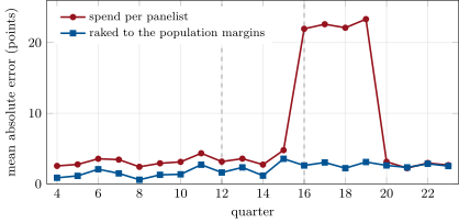
A card-spending panel nowcasts a hundred retailers’ year-on-year sales growth within 3.3 percentage points on average for three years; in the fourth it misses by 22.5. Nothing changed at the retailers. The vendor had changed its bank partner, and the new partner’s cardholders were older and lived elsewhere. Book 7 (chapter 12) taught how to decide whether to buy a dataset; Book 8 (chapter 16) traded one. This chapter is the plumbing in between, where most of the work and most of the losses are: ingesting deliveries that are sometimes wrong, turning merchant strings into securities, correcting a panel that is not the population, and telling a history the vendor lived through from one it reconstructed. Every number comes from a synthetic panel whose truth is known, built so that each stage has something to catch.

15.1 Ingestion and validation

Definition 15.1 (Ingestion pipeline, schema validation)

An ingestion pipeline is the code that receives a vendor’s deliveries, checks them, maps them to the firm’s identifiers and stores them with the time each value became known. Schema validation checks each record against a declared schema: every field present, of its type and in its range, and no record duplicated; records that fail are rejected with a reason, never silently repaired.

The chapter’s world has 100 retailers over 24 quarters. Their true sales are spent by a population divided into six cells, three age bands by two regions, with known shares; each retailer draws its customers from the cells in its own proportions, and spending in each cell grows at its own rate. The vendor’s panel holds 50 000 cardholders from one bank, tilted young (45% in the youngest band against 30% of the population) and drifting younger by a point a quarter; at quarter 16 the vendor changes partner and the panel becomes 30 000 cardholders, half in the oldest band and three-quarters in one region. The vendor launches at quarter 12, delivering quarters 0 to 11 at once, then one quarter’s data a quarter after it ends.

Each delivery is rows of quarter, merchant string, age band, region, spend and panel count, one retailer’s spend in a cell split across two or three store-level strings: 36 766 rows in all, with planted defects. Schema validation (Listing 15.1) rejects 121 rows with a missing field, 69 with a negative spend, 64 with the panel count delivered as text, and 111 duplicates, every planted defect and nothing else. A row can be valid and the delivery wrong: the delivery for quarter 19 arrives in cents. A second check compares each delivery’s total with the previous one and holds it for review when the ratio leaves $[0.5, 2]$ ; it holds that delivery and no other, and review rescales it. Checks on the delivery, not only on the rows, are what catch a vendor’s change of units, a lost file or a file sent twice.

15.2 Mapping to securities

Definition 15.2 (Entity resolution, record linkage)

Record linkage decides which records in two files describe the same entity when no common identifier exists, by comparing their attributes (Fellegi and Sunter, 1969). Entity resolution is the task applied to a dataset’s entity strings (merchants, issuers, apps, vessels) against a reference list, here the security master (Book 7, chapter 4): normalise, compare, and decide to match, to send to review, or to leave unmatched.

A card network prints “SQ *BOREALIS RET”, “BOREALIS RETAIL #4417”, “BOREALI RETA STR 313” or “BOREALIS 5120”, and the model needs the permanent identifier of Borealis Retail, not a string. The resolver of Listing 15.2 strips processor prefixes, store numbers and filler words, then scores each alias by its tokens, counting a token found as a prefix of three letters or more (card networks truncate) as a full match. Of the 600 strings of the retailers, exact matching on the normalised name finds 300; the resolver matches 500 automatically, all correctly, and sends the other 100 to review: the strings that give only the name’s first word, which up to three retailers share (Borealis Retail, Borealis Stores, Borealis Outfitters). Of ten strings from unrelated merchants (“DELTA AIR LINES”, “SUMMIT DENTAL CARE”), none is matched, six go to review and four are rejected outright. The review queue is where a person earns their place in the pipeline: matching a store to the wrong retailer contaminates its sales silently, while a string left for review only delays it.

15.3 Panel bias and reweighting

Definition 15.3 (Panel bias, panel reweighting)

Panel bias is the difference between a statistic computed on a data vendor’s panel (cardholders, devices, users) and the same statistic on the population it stands for, caused by who is in the panel. Panel reweighting gives each panel member a weight so that the weighted panel matches known population totals; raking (iterative proportional fitting) does it with only the margins, adjusting the weights to each margin in turn until all match (Deming and Stephan, 1940).

The raw nowcast divides each retailer’s panel spend by the number of panelists and reads year-on-year growth from it. While the panel drifts slowly, the error is modest (3.3 points on average over quarters 4 to 15): a retailer whose young customers spend more each year looks, in a panel getting younger, as if it grows faster than it does. In the four quarters after the partner change, each year-on-year comparison sets the new panel against the old, and the error jumps to 22.5 points (Figure 15.1); it returns to 2.7 once both sides of the comparison come from the new panel. Raking the six cells to the population’s age and region margins (Listing 15.3) removes the composition effect: 1.7 points before the change, 2.7 in the change year, 2.6 after. The change year’s residual comes from the new panel’s small cells (1 125 cardholders in the thinnest), whose sampling noise no reweighting removes.

Mean absolute error, across 100 retailers, of the year-on-year sales growth read from the panel. Dashed: the vendor’s launch (quarter 12) and its change of bank partner (quarter 16). Data: ml_altdata.errors. — **Figure 15.1.** Mean absolute error, across 100 retailers, of the year-on-year sales growth read from the panel. Dashed: the vendor’s launch (quarter 12) and its change of bank partner (quarter 16). Data: `ml_altdata.errors`.

Raking needs the population margins to be known and the panel to cover every cell: a cell the panel does not reach cannot be reweighted into existence. It also assumes that within a cell the panel spends like the population, which is the assumption a new partner is most likely to break (its cardholders may be richer as well as older). The vendor’s own reweighting, when there is one, deserves the same scrutiny as the raw panel: ask for the margins it rakes to and for the panel’s composition by quarter.

15.4 Detecting backfill

Definition 15.4 (First-seen timestamp)

The first-seen timestamp of a value is the time the firm first received it, recorded by the firm at ingestion, as opposed to the valid time the vendor attaches to it. A value whose first-seen time is much later than its valid time was backfilled (Book 7, chapter 3), and its history cannot be trusted to be what a live user would have seen.

The pipeline stores every value in the bitemporal store of Book 7 (chapter 3), with the delivery quarter as knowledge time, and the backfill test is one query: quarters 0 to 10 were first seen at quarter 12, more than a quarter after they ended. They matter because the vendor built them at launch with hindsight, moving its panel estimates three quarters of the way towards the sales the retailers had already reported. (Quarter 11, delivered at launch one quarter after it ended, looks like a live quarter and was not adjusted: its sales had not yet been reported.)

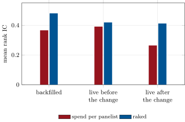
To score the nowcast as a predictor, each retailer’s announcement return is its sales surprise, true growth minus a consensus that misses by 3 points on average, plus noise. The rank information coefficient between the raked nowcast’s surprise and the return is 0.480 on the backfilled quarters and 0.419 on the live quarters before the partner change, 0.412 after it (Figure 15.2). The raw nowcast’s IC falls from 0.391 live before the change to 0.264 after it. A trial that scores the backfilled history, which is most of what a new vendor can offer, sees a signal about 15% stronger than the one it will trade.

Mean rank information coefficient of the nowcast’s surprise with the announcement return, by period. Data: ml_altdata.ic_summary. — **Figure 15.2.** Mean rank information coefficient of the nowcast’s surprise with the announcement return, by period. Data: `ml_altdata.ic_summary`.

15.5 From pipeline to predictor

The nowcast becomes a predictor through the vendor-trial harness of Book 7 (chapter 12): coverage by quarter, the backfill share, a panel-drift test on the residuals against reported sales, the IC by year and the incremental IC over what the desk already owns. The pipeline’s job is to hand it data that mean what they say. Froot, Kang, Ozik and Sadka (2017) built real-time sales proxies for retailers from about 50 million mobile devices and related them to earnings surprises and announcement returns; Katona, Painter, Patatoukas and Zeng (2024) used the introduction of satellite coverage of retailers’ car parks to show that investors with such data traded profitably ahead of retailers’ reports, especially bad ones. Both depend on the plumbing this chapter builds: which stores belong to which company, who is in the panel, and when each number was known.

Method 15.5 (An alternative-data pipeline)

Validate every row against a schema and every delivery against the last; reject with reasons, hold what looks wrong, never repair silently.
Resolve entities to permanent identifiers with a match threshold, a review band and a person on the queue; measure precision on a labelled sample.
Store every value with its first-seen time; label backfill; score trials on live data only.
Obtain the panel’s composition by period and rake it to known margins; monitor composition for breaks.
Hand the result to the trial harness and, once live, to monitoring (chapter 27).

15.6 Tutorial: the panel that grew

Goal. Ingest a vendor’s deliveries, resolve its merchant strings, rake its panel and compare nowcast errors and ICs by period. End state: Figures 15.1 and 15.2.

Schema validation.

def validate(rows, schema=SCHEMA):
    """Keep the rows whose every field is present, of the right type and in range; drop exact duplicates."""
    clean, rejects, seen = [], [], set()
    for r in rows:
        reason = None
        for f, (typ, ok) in schema.items():
            v = r.get(f)
            if v is None:
                reason = f"missing {f}"
            elif not isinstance(v, typ) or isinstance(v, bool):
                reason = f"type {f}"
            elif not ok(v):
                reason = f"range {f}"
            if reason:
                break
        key = tuple(r.get(f) for f in schema)
        if reason is None and key in seen:
            reason = "duplicate"
        if reason:
            rejects.append((r, reason))
        else:
            seen.add(key)
            clean.append(r)
    return clean, rejects

Listing 15.1. Row validation against a schema. code/firm/altdata/firm_altdata.py

Merchant strings to identifiers.

def similarity(a, b):
    """Token-level match of a merchant string a against an alias b: each alias token scores 1 if some token of a is
    equal to it or a prefix of it of at least three letters (card networks truncate), else its best character-level
    ratio; the score is the mean over the alias's tokens, less a penalty for tokens of a that match nothing."""
    ta, tb = a.split(), b.split()
    if not ta or not tb:
        return 0.0

    def tok(x, y):
        if x == y or (len(x) >= 3 and y.startswith(x)):
            return 1.0
        return difflib.SequenceMatcher(None, x, y).ratio()

    cover = float(np.mean([max(tok(x, y) for x in ta) for y in tb]))
    extra = sum(max(tok(x, y) for y in tb) < 0.8 for x in ta) / len(ta)
    return cover * (1 - 0.5 * extra)


def resolve(strings, aliases, accept=0.9, review=0.5):
    """aliases: {alias text: pid}. Each merchant string is normalised and compared with every normalised alias; the best
    score above `accept` is a match, between `review` and `accept` goes to a person, below is unmatched. A tie between
    two companies above `review` also goes to review."""
    norm = [(normalise(a), pid) for a, pid in aliases.items()]
    out = {}
    for s in strings:
        n = normalise(s)
        scored = sorted(((similarity(n, a), pid) for a, pid in norm), reverse=True)
        best, pid = scored[0]
        rival = next((sc for sc, p in scored[1:] if p != pid), 0.0)
        if best >= accept and best - rival > 1e-9:
            out[s] = (pid, best, "matched")
        elif best >= review:
            out[s] = (pid, best, "review")
        else:
            out[s] = (None, best, "none")
    return out

Listing 15.2. Token similarity and resolution with a review band. code/firm/altdata/firm_altdata.py

Raking.

def rake(counts, row_margin, col_margin, iters=50):
    """Iterative proportional fitting: weights w (cells, same shape as counts) such that the weighted counts' row sums
    match row_margin and column sums match col_margin (margins as shares or totals, rescaled to the panel's total)."""
    counts = np.asarray(counts, dtype=float)
    tot = counts.sum()
    r = np.asarray(row_margin, float) / np.sum(row_margin) * tot
    c = np.asarray(col_margin, float) / np.sum(col_margin) * tot
    w = np.ones_like(counts)
    for _ in range(iters):
        w *= (r / (w * counts).sum(1))[:, None]
        w *= (c / (w * counts).sum(0))[None, :]
    return w

Listing 15.3. Iterative proportional fitting to two margins. code/firm/altdata/firm_altdata.py

Run ml_altdata.ingest(), resolution_quality(), error_summary(), ic_summary() and fig_altdata.py.

What to change next. Give the new partner’s cardholders a different spending level within each cell, and watch raking fail; lower the review threshold and count the wrong matches.

15.7 Build: the alternative-data pipeline

Purpose. Vendor deliveries turned into point-in-time, identifier-keyed, reweighted data a predictor can use.

Interface. SCHEMA, validate(rows, schema), delivery_check(prev, new, lo, hi); normalise, similarity, resolve(strings, aliases, accept, review); rake(counts, row_margin, col_margin, iters); first_seen(store, entity, field, valid) on firm.pit; card_panel(n_firms, quarters, launch, partner_change, seed).

Rules. Rejections carry reasons; nothing is repaired without a record; every stored value has a knowledge time; matches below the threshold wait for a person.

Acceptance tests. code/firm/altdata/tests/: each defect type is rejected with its reason and clean rows pass; a doubled delivery is held; truncated and prefixed strings resolve, shared stems go to review, unrelated merchants do not match; raking matches both margins and leaves a panel already at the margins unweighted; first-seen times separate a backfilled history.

Stretch. Fellegi–Sunter match weights learned from the review decisions; raking to three margins with a cap on weights; the panel’s composition monitored for breaks.

Sources and further reading

I. P. Fellegi and A. B. Sunter, “A theory for record linkage”, Journal of the American Statistical Association 64(328), 1969.
W. E. Deming and F. F. Stephan, “On a least squares adjustment of a sampled frequency table when the expected marginal totals are known”, Annals of Mathematical Statistics 11(4), 1940.
K. A. Froot, N. Kang, G. Ozik and R. Sadka, “What do measures of real-time corporate sales say about earnings surprises and post-announcement returns?”, Journal of Financial Economics 125(1), 2017.
Z. Katona, M. Painter, P. N. Patatoukas and J. Zeng, “On the capital market consequences of big data: evidence from outer space”, Journal of Financial and Quantitative Analysis, 2024.

15.8 Exercises

Exercise 15.1 ★

A delivery totals 2.4 billion; the previous one totalled 23.9 million. What does the delivery check do, and what are the likely causes?

Solution

Solution of Exercise 15.1.

The ratio is about 100, far outside $[0.5, 2]$ : the delivery is held for review. A factor of 100 points to a change of units (cents for dollars); other causes of a large ratio are a file delivered twice, a new partner’s data added, or cumulative totals sent instead of increments.

Exercise 15.2 ★

Rake the $2\times2$ panel counts $\begin{pmatrix}30 & 20\\ 10 & 40\end{pmatrix}$ to even row and column margins. Give the weighted counts.

Solution

Solution of Exercise 15.2.

Weights $\begin{pmatrix}1.18 & 0.72\\ 1.45 & 0.89\end{pmatrix}$ (to two decimals), weighted counts $\begin{pmatrix}35.5 & 14.5\\ 14.5 & 35.5\end{pmatrix}$ : every row and column sums to 50. Raking matches the margins, not the cells; many weightings do, and raking picks the one closest to the starting weights in a relative-entropy sense.

Exercise 15.3 ★

Why does “BOREALIS 5120” go to review while “BOREALI RETA STR 313” is matched?

Solution

Solution of Exercise 15.3.

“BOREALIS 5120” normalises to “borealis”, which matches the first token of three retailers’ names equally (Borealis Retail, Stores and Outfitters) and none of their second tokens: score 0.79 for each, a tie in the review band. “BOREALI RETA STR 313” normalises to “boreali reta”, whose tokens are prefixes of “borealis” and “retail”: score 1 for Borealis Retail alone.

Exercise 15.4 ★★

Explain, with the chapter’s world, why the raw nowcast’s error rises for exactly four quarters after the partner change.

Solution

Solution of Exercise 15.4.

Year-on-year growth compares a quarter with the same quarter a year earlier. For quarters 16 to 19 the current value comes from the new panel and the earlier one from the old, so the change in who is in the panel is read as a change in sales, by an amount that depends on each retailer’s customers. From quarter 20 both sides come from the new panel, and the error returns to the level of a stable panel (2.7 points).

Exercise 15.5 ★★

Why could the first-seen test not flag quarter 11, and why did that not matter here? When would it?

Solution

Solution of Exercise 15.5.

It was delivered at launch one quarter after it ended, exactly like a live quarter, so its timestamps are indistinguishable from live data. It did not matter because the vendor could not adjust it: the retailers had not yet reported its sales. It would matter if the vendor had built it with any later information (a merchant map fitted afterwards, a panel cleaned of later dropouts), which only the vendor’s documentation or a comparison of vintages can reveal.

Exercise 15.6 ★★

Find the flaw. “We fixed the vendor’s negative spends by taking absolute values and cast the text panel counts to integers, so no data were lost.”

Solution

Solution of Exercise 15.6.

Repairing hides the vendor’s problem and guesses the fix: a negative spend may be a refund, a sign error or a corrupted row, and its absolute value is only one guess. Reject, count by reason, report to the vendor, and repair only with a rule the vendor confirms, recorded with the data.

Exercise 15.7 ★★★

Coding. Run the pipeline with the review queue left unresolved (strings in review dropped). What happens to the raked nowcast’s error, and why is the error larger for some retailers than others?

Solution

Solution of Exercise 15.7.

The raked error rises from 2.1 to 19.7 points on average. The dropped strings carried 18.4% of the retailers’ delivered spend, but in a share that changes from quarter to quarter (each cell’s spend is split at random across two or three of a retailer’s strings), so dropping them adds noise to every growth rate rather than a constant bias. Retailers and quarters where the stem-only string happened to carry more spend suffer most.

Exercise 15.8 ★★★

Show that with a panel whose cell counts are the product of an age margin and a region margin, raking to the population’s margins gives the post-stratification weights (population share over panel share of each cell) when the population’s cell shares are also a product. What happens when they are not?

Solution

Solution of Exercise 15.8.

Let the panel’s cell counts be $n_{ar} = N u_a v_r$ and the population’s shares $p_{ar} = \alpha_a\beta_r$ . The weights $w_{ar} = (\alpha_a/u_a)(\beta_r/v_r)$ give weighted counts $N\alpha_a\beta_r$ , which match both margins, and raking’s first two steps reach them: the row step multiplies by $\alpha_a/u_a$ , after which the column sums are $N\alpha_\cdot v_r$ and the column step multiplies by $\beta_r/v_r$ . These are the post-stratification weights $p_{ar}/(n_{ar}/N)$ . When the population has an interaction ( $p_{ar}\ne\alpha_a\beta_r$ ), raking still matches the margins but not the cells, and a statistic that depends on the interaction stays biased.

15.9 Problem: The Panel That Grew

Problem 15.1

Weekend problem — a panel is not a population

The chapter’s world: 100 retailers, 24 quarters, a panel that drifts, changes partner at quarter 16 and launches at quarter 12 with a backfilled history.

Part I — Ingestion.

What defects were planted, and how many rows does validation reject?
Which defect does row validation miss, and what catches it?
Why reject rather than repair?
What does the pipeline store for each value, and why?

Part II — Resolution.

How many strings does exact matching resolve, and how many the resolver?
What goes to review, and why is that the right place for it?
What happens to the unrelated merchants?
What does a wrong match cost, compared with a string left in review?

Part III — Panel and backfill.

What are the raw and raked nowcast errors before, during and after the change year?
What does raking assume, and what residual error remains?
Which quarters are backfilled, and how does the pipeline know?
What are the ICs on backfilled and live history?

Part IV — The verdict.

State the named result: the nowcast error with and without reweighting after the partner change, and the IC of the backfilled history against the live one.
What would you ask a card-panel vendor for before a trial?
How would you detect a partner change the vendor did not announce?
What would you monitor once the data are live?
How much of the backfilled IC would you believe?
Where would a person sit in this pipeline, and why there?
What changes for a satellite or app-download panel?
In one sentence: what is the most expensive assumption in alternative data?

Solution

Solution of Problem 15.1.

Part I.

Missing fields, negative spends, panel counts as text, duplicated rows, and one delivery in cents. Validation rejects 121, 69, 64 and 111 rows, every planted defect.
The delivery in cents: every row is valid. The delivery check against the previous total holds it.
A repair is a guess about the vendor’s error; rejection keeps the data honest and makes the vendor fix it.
The value with its valid time and the delivery time as knowledge time, so that every query can be asked as of a date and backfill can be seen.

Part II.

Exact matching on the normalised name: 300 of 600. The resolver: 500 matched automatically, all correctly, 100 to review, none unmatched.
The strings with only a first word that up to three retailers share: a machine cannot tell them apart and a person with store lists can.
None is matched; six go to review, four are rejected.
A wrong match moves spend between companies silently and biases both nowcasts; a string in review delays data and costs a person’s time.

Part III.

Raw: 3.3 points (quarters 4–15), 22.5 (16–19), 2.7 (20–23). Raked: 1.7, 2.7, 2.6.
That population margins are known, that the panel covers every cell, and that within a cell panelists spend like the population. The residual is sampling noise in small cells and any within-cell difference.
Quarters 0 to 10: their first-seen time is quarter 12, more than a quarter after they ended.
Raked: 0.480 backfilled, 0.419 live before the change, 0.412 after. Raw: 0.366, 0.391, 0.264.

Part IV.

The panel that grew. In the year after the partner change the raw nowcast misses growth by 22.5 points on average, the raked one by 2.7; the backfilled history’s IC is 0.480 against 0.419 live.
The panel’s composition by period and the margins it is weighted to; partner and methodology changes with dates; delivery timestamps for all history; the merchant map and its changes.
A break in composition (panel counts by cell), in the relation of panel totals to reported sales (Book 7’s CUSUM on residuals), and a jump in the share of new merchant strings.
Delivery checks, rejection rates, the review queue, panel composition, nowcast residuals against reported sales, and the live IC.
None of the difference from live; treat backfilled history as an upper bound and plan on the live number.
On the review queue and on held deliveries: where the machine’s uncertainty is concentrated and a person’s knowledge is cheapest.
The same stages with other entities (sites, vessels, apps) and other biases (cloud cover, device mix, store openings); the composition question and the first-seen question do not go away.
That the panel still represents the population it represented when the model was fitted.

15.10 Interview questions

Interview question 15.1 ★ researcher, mle

What is backfill in a vendor dataset, and how do you detect it?

Solution

Solution of Interview question 15.1.

History delivered after the fact, often built with information unavailable at the time (a merchant map, calibration to reported numbers). Detect it by recording first-seen timestamps at ingestion, asking the vendor for delivery dates and vintages, and comparing the history’s statistics with the live period’s.

What the interviewer is looking for: the definition, first-seen timestamps, and live-versus-backfill comparison.

Interview question 15.2 ★★ mle, developer

Design the ingestion step for a daily vendor file. What do you check, and what do you do when a check fails?

Solution

Solution of Interview question 15.2.

Schema (fields, types, ranges, uniqueness), delivery-level checks (row counts, totals against the last delivery, coverage, arrival time), and referential checks (unknown entities). On failure: reject rows with reasons, hold the delivery, alert, never repair silently; store with knowledge times.

What the interviewer is looking for: row and delivery checks, and a failure policy with no silent repair.

Interview question 15.3 ★★ mle

How would you map merchant descriptors to listed companies at scale, and how would you measure the mapping’s quality?

Solution

Solution of Interview question 15.3.

Normalise descriptors, block candidates by tokens, score by token and prefix similarity (or a trained matcher), accept above a threshold, review a band, reject below; keep the mapping point in time. Measure precision and recall on a labelled sample, stratified by descriptor pattern, and track the review queue and new-string rates.

What the interviewer is looking for: thresholds with review, point-in-time mapping, measured precision.

Interview question 15.4 ★★ researcher

A card panel over-represents young customers. How do you correct a sales nowcast for it, and what can go wrong?

Solution

Solution of Interview question 15.4.

Reweight the panel to population margins (raking or post-stratification) by age and other known dimensions. It fails when cells are empty or tiny, when margins are unknown or stale, when panelists differ from the population within cells, and when composition changes break year-on-year comparisons.

What the interviewer is looking for: reweighting and its assumptions, including within-cell differences.

Interview question 15.5 ★★ researcher, trader

A nowcast that tracked sales for three years misses badly for a year. What do you check first?

Solution

Solution of Interview question 15.5.

The data before the model: a change of partner or methodology, panel composition, the merchant map, delivery timing; then the retailer (a new channel the panel does not see, such as online sales through another processor); only then the model.

What the interviewer is looking for: panel and mapping changes before model changes.

Interview question 15.6 ★★★ researcher

A vendor’s trial shows an IC of 0.5 over eight years; the dataset launched two years ago. How would you estimate the IC you should expect live?

Solution

Solution of Interview question 15.6.

Split the trial at launch: the two live years are the evidence, with their standard error; the six backfilled years are an upper bound. Check the vendor’s backfill method, compare vintages, and shrink the estimate towards the live IC; expect further decay as others buy the data (Book 8, chapter 16).

What the interviewer is looking for: live-only estimation, skepticism of backfill, and expected decay.

Terms defined in this chapter

See all 2333 terms in the glossary