Machine Learning for Markets · Machine learning

9Cross-Sectional Deep Models

A statistical factor model extracts three factors from a panel of stock returns and gives each stock a fixed loading on each. A stock listed yesterday has no loading; a stock whose characteristics have changed keeps the loading of the stock it was. On a simulated panel whose true betas are functions of ten characteristics, half of their variation nonlinear, the loadings of principal-component analysis explain 22.5% of the test months’ returns, and their expected returns correlate at 0.03 with the true ones. Betas written as linear functions of the characteristics (instrumented PCA) explain 27.6% and correlate at 0.71; betas written as a small neural network of them (a conditional autoencoder) explain 30.4% and correlate at 0.95, against a ceiling of 31.3%. This chapter builds models that learn from a panel as a panel: pooled across assets, with inputs that describe the asset rather than name it.

9.1 Panels, pooling and permutation invariance

Definition 9.1 (Pooled panel model, permutation-invariant network)

A pooled panel model fits one function $f_\theta(x_{it})$ to every asset $i$ and date $t$ of a panel, so that assets share parameters through their characteristics rather than each having its own. A permutation-invariant network maps a set of vectors to an output that does not depend on their order, typically $\rho(\sum_i\phi(x_i))$ for networks $\phi$ and $\rho$ (Zaheer et al., 2017).

Every model of chapters 4 to 7 was pooled: one ridge regression or one network for all 500 stocks. Pooling is what makes a panel of 500 stocks and 240 months a large dataset; its price is the assumption that stocks with the same characteristics behave alike, which is exactly what a factor model with characteristic-driven betas says. Permutation invariance appears as soon as a model needs the whole cross-section as an input: the average of any characteristic over the stocks, or a characteristic-weighted portfolio’s return, does not depend on how the stocks are ordered, and it is how the models below turn a cross-section of any size into a fixed number of factors.

9.2 Embeddings for identifiers and categories

Definition 9.2 (Entity embedding)

An entity embedding represents each value $j$ of a categorical variable (an industry, a venue, a stock identifier) by a vector $e_j\in\mathbb R^m$ learned with the rest of the network, in place of a one-hot column per category (Guo and Berkhahn, 2016).

Thirty industries are planted on top of the chapter’s panel, each with a monthly premium drawn with a standard deviation of 0.4%. A pooled network on the ten characteristics alone explains 0.004% of the test months’ demeaned returns; with a one-dimensional embedding of the industry it explains 0.15%, its forecasts’ correlation with the true expected returns rises from 0.52 to 0.75, and the learned embedding correlates at 0.86 with the planted premia (the industries’ raw average returns over the training months correlate at 0.88). One practical detail decided the result: embeddings initialised with PyTorch’s default standard deviation of one never moved far enough from their random start for the premia to show; initialised near zero (standard deviation 0.01), they learned them.

9.3 Learned factor models: instrumented PCA and conditional autoencoders

The chapter’s panel is firm.mlsynth.factor_panel: 300 stocks, 240 months, ten ranked characteristics, three factors with monthly premia of 0.6%, 0.4% and 0.3%, and betas that are functions of the characteristics, half of their cross-sectional variance linear and half nonlinear (squares, products, absolute values). The truth’s expected return is $\mu_{it} = \beta(z_{it})^\top\lambda$ .

Definition 9.3 (Instrumented principal component analysis)

Instrumented principal component analysis (IPCA) models $r_{i,t+1} = z_{it}^\top\Gamma f_{t+1} + e_{i,t+1}$ with $K$ latent factors $f$ and betas $z^\top\Gamma$ linear in the characteristics (a constant included); $\Gamma$ ( $L\times K$ ) and the factors are estimated by alternating least squares, the factors month by month as cross-sectional regressions of returns on $Z_t\Gamma$ (Kelly, Pruitt and Su, 2019).

Definition 9.4 (Autoencoder, conditional autoencoder)

An autoencoder is a network trained to reproduce its input through a lower-dimensional bottleneck: an encoder maps $x$ to a code $h$ , a decoder maps $h$ back to $\hat x$ , and the loss is the reconstruction error. A conditional autoencoder reconstructs the cross-section of returns $r_{t+1}$ as $\beta(z_{it})^\top f_{t+1}$ , where the code $f_{t+1}$ ( $K$ factors) is a linear map of characteristic-managed portfolios $Z_t^\top r_{t+1}/n$ and the betas are a network of the characteristics (Gu, Kelly and Xiu, 2021).

The managed portfolios are the permutation-invariant summary of the cross-section: their number is the number of characteristics, whatever the number of stocks. The chapter’s autoencoder has a beta network with two hidden layers (32 and 16 units) and a linear factor map; it is trained on months 0 to 159 with early stopping on months 160 to 179; IPCA and PCA are fitted on months 0 to 179; all three are scored on months 180 to 239.

Proposition 9.5 (Why IPCA is a regression)

For fixed $\Gamma$ , the least-squares factors of month $t$ are $\hat f_{t+1} = (\Gamma^\top Z_t^\top Z_t\Gamma)^{-1}\Gamma^\top Z_t^\top r_{t+1}$ ; for fixed factors, $\operatorname{vec}(\Gamma^\top)$ solves the normal equations $\sum_t(Z_t^\top Z_t\otimes f_{t+1}f_{t+1}^\top)\operatorname{vec}(\Gamma^\top) = \sum_t(Z_t^\top r_{t+1})\otimes f_{t+1}$ .

Proof. The first is ordinary least squares of $r_{t+1}$ on the columns of $Z_t\Gamma$ . For the second, $z_{it}^\top\Gamma f = (z_{it}\otimes f)^\top\operatorname{vec}(\Gamma^\top)$ , a linear model in $\operatorname{vec}(\Gamma^\top)$ whose normal equations sum $(z\otimes f)(z\otimes f)^\top = zz^\top\otimes ff^\top$ over assets and months. ∎

9.4 Evaluating a learned factor model

Two R-squared measure a factor model (Kelly, Pruitt and Su; Gu, Kelly and Xiu). The total R-squared uses the month’s realised factors: how much of the cross-section’s variation the betas can explain once the factors are known. The predictive R-squared uses the average factor of the training months, $\beta^\top\hat\lambda$ : an expected-return forecast. Both are measured against zero.

	total $R^2$			3 factors: corr. of $\hat\mu$ with
model	1 factor	3 factors	5 factors	the truth $\mu$	$\mu$ ’s nonlinear part
PCA (static betas)	22.0%	22.5%	23.0%	0.03	0.00
IPCA (linear betas)	25.1%	27.6%	28.1%	0.71	$-0.03$
conditional autoencoder	26.9%	30.4%	30.8%	0.95	0.59
the truth	31.3%			1

Table 9.1. Three factor models on the sixty test months of the conditional factor panel. Total R-squared uses realised factors; the last two columns correlate each model’s expected returns

\beta^\top\hat\lambda

with the true

\mu

and with the part of

\mu

that comes from the betas’ nonlinear terms. Autoencoder: seed 1; seeds 2 and 3 give 30.5% and 30.6% total and correlations of 0.95 and 0.96. Data: ml_xsnet.

Table 9.1 has three findings. Static betas are the wrong model for a panel whose characteristics move: PCA’s expected returns carry no cross-sectional information (correlation 0.03), although its total R-squared, driven by the market factor, is respectable. Linear betas recover the linear part of the truth and none of the nonlinear part ( $-0.03$ ). The autoencoder recovers both, most of the way (0.95 overall, 0.59 of the nonlinear part), and its total R-squared is within a point of the truth’s with three factors. The predictive R-squared, 1.01% for PCA, 1.11% for IPCA and 1.23% for the autoencoder against 1.09% for the truth itself, ranks the models the same way but should not be read alone: over sixty months it is dominated by the level of the premia and by how the test window’s factor returns happened to average, which is why the truth can be beaten on it.

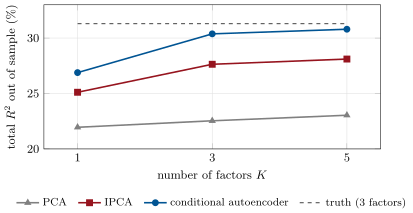
Total R-squared of the test months against the number of factors. The truth has three factors; the models with more have more room to fit, not more truth to find. Data: ml_xsnet.pca, ipca, cae. — **Figure 9.1.** Total R-squared of the test months against the number of factors. The truth has three factors; the models with more have more room to fit, not more truth to find. Data: `ml_xsnet.pca`, `ipca`, `cae`.

Method 9.6 (Fitting a learned factor model)

Rank the characteristics by date and add a constant; keep the return of month $t+1$ with the characteristics of month $t$ .
Fit IPCA first: it is fast, has no seeds, and tells how much a linear-beta model explains.
Fit the conditional autoencoder with early stopping on held-out months and several seeds; compare with IPCA on total R-squared and on the correlation of expected returns with a benchmark forecast.
Choose the number of factors on held-out months; report both R-squared and never the predictive one alone.

9.5 Tutorial: factors that learn

Goal. Fit PCA, IPCA and a conditional autoencoder with one, three and five factors on a panel with characteristic-driven betas; measure how much of the planted nonlinearity each recovers; add industries through an embedding. End state: Table 9.1, Figure 9.1.

IPCA by alternating least squares (Proposition 9.5).

    def factors(self, Z, r):
        G = self.G
        return np.stack([np.linalg.solve(G.T @ z.T @ z @ G, G.T @ z.T @ x) for z, x in zip(Z, r, strict=True)])

    def fit(self, Z, r):
        X = managed(Z, r)
        _, _, vt = np.linalg.svd(X, full_matrices=False)
        self.G = vt[: self.K].T
        L, K = self.G.shape
        for _ in range(self.iters):
            F = self.factors(Z, r)
            A = np.zeros((L * K, L * K))
            b = np.zeros(L * K)
            for z, x, f in zip(Z, r, F, strict=True):
                A += np.kron(z.T @ z, np.outer(f, f))
                b += np.kron(z.T @ x, f)
            G = np.linalg.solve(A, b).reshape(L, K)
            q, _ = np.linalg.qr(G)                                      # Gamma' Gamma = I
            self.G = q
        F = self.factors(Z, r)
        w, V = np.linalg.eigh(F.T @ F)
        self.G = self.G @ V[:, ::-1]
        self.lam = self.factors(Z, r).mean(axis=0)
        return self

Listing 9.1. Instrumented PCA: factors by cross-sectional regression, loadings by the Kronecker normal equations. code/firm/xsnet/firm_xsnet.py

The conditional autoencoder: betas from characteristics, factors from managed portfolios.

class _CA(nn.Module):
    def __init__(self, L, K, hidden):
        super().__init__()
        layers, d = [], L
        for h in hidden:
            layers += [nn.Linear(d, h), nn.ReLU()]
            d = h
        self.beta = nn.Sequential(*layers, nn.Linear(d, K))
        self.fac = nn.Linear(L, K, bias=False)

    def forward(self, z, x):                                            # z: (m, n, L), x: (m, L)
        return torch.einsum("mnk,mk->mn", self.beta(z), self.fac(x))

Listing 9.2. The conditional autoencoder’s two networks. code/firm/xsnet/firm_xsnet.py

Run ml_xsnet.pca(K), ipca(K), cae(K, seed), embedding() and fig_xsnet.py.

What to change next. Set the planted nonlinear share to zero and check that IPCA catches up with the autoencoder; give the autoencoder’s factor map the managed portfolios of squared characteristics too.

9.6 Build: cross-sectional networks and factor models

Purpose. The firm’s learned factor models, comparable on one panel and one pair of R-squared.

Interface. managed(Z, r), with_constant(Z), PCAModel(K), IPCA(K, iters) with fit, factors, betas, score; CondAE(L, K, hidden, seed) with the same methods; scores(pred_total, pred_mu, r); EmbedMLP, fit_embed.

Rules. Characteristics of month $t$ with returns of month $t+1$ ; managed portfolios computed with the same month’s characteristics and returns; one CPU thread, early stopping on held-out months.

Acceptance tests. code/firm/xsnet/tests/: IPCA recovers a planted linear-beta model’s betas (up to rotation) and its alternating steps never increase the loss; PCA recovers static loadings; the autoencoder’s managed-portfolio input is invariant to reordering the stocks; an embedding recovers planted category effects.

Stretch. IPCA with an intercept (alpha) test; the autoencoder with nonlinear factor maps; the no-arbitrage criterion of Chen, Pelger and Zhu.

Sources and further reading

B. Kelly, S. Pruitt and Y. Su, “Characteristics are covariances: a unified model of risk and return”, Journal of Financial Economics 134(3), 2019.
S. Gu, B. Kelly and D. Xiu, “Autoencoder asset pricing models”, Journal of Econometrics 222(1), 2021.
L. Chen, M. Pelger and J. Zhu, “Deep learning in asset pricing”, Management Science 70(2), 2024.
C. Guo and F. Berkhahn, “Entity embeddings of categorical variables”, arXiv, 2016.
M. Zaheer et al., “Deep sets”, NeurIPS, 2017.

9.7 Exercises

Exercise 9.1 ★

With ten characteristics plus a constant and three factors, how many parameters has IPCA’s $\Gamma$ ? How many has a static PCA model of 300 stocks with three factors?

Solution

Solution of Exercise 9.1.

$\Gamma$ is $11\times3$ : 33 parameters, whatever the number of stocks. Static PCA: $300\times3 = 900$ loadings, and a stock without history has none.

Exercise 9.2 ★

Three stocks have characteristic values 0.5, $-0.5$ , 1.0 and returns 2%, $-1\%$ , 3% in a month. What is the characteristic’s managed-portfolio return, and does it depend on the order of the stocks?

Solution

Solution of Exercise 9.2.

$(0.5\times2 + (-0.5)(-1) + 1.0\times3)/3 = 1.5\%$ . A sum over stocks does not depend on their order.

Exercise 9.3 ★

Thirty industries, a one-hot encoding into a hidden layer of 32 units against a one-dimensional embedding feeding the same layer: how many parameters does each use for the industry?

Solution

Solution of Exercise 9.3.

One-hot into 32 units: $30\times32 = 960$ weights. A one-dimensional embedding: 30 values plus 32 weights from the embedding to the layer, 62 in all.

Exercise 9.4 ★★

Why does PCA’s expected return carry no cross-sectional information on this panel, although its total R-squared is 22.5%?

Solution

Solution of Exercise 9.4.

PCA’s loadings are averages of each stock’s betas over the training years, while the betas move with the characteristics: by the test months the stocks’ current betas, and so their expected returns, have little to do with those averages (correlation 0.03). The total R-squared comes mostly from the first factor, a market factor with betas near one, which any loading captures.

Exercise 9.5 ★★

Why can a model beat the truth on predictive R-squared over sixty months, and what should be reported instead?

Solution

Solution of Exercise 9.5.

Predictive R-squared against zero is driven by the level of the forecast relative to the realised mean return; over sixty months the realised factor means differ from the premia, and a model whose average forecast happens to match them better scores higher than the truth (1.23% against 1.09%). Report total R-squared, the correlation of expected returns with the truth (on simulated data) or with realised returns (the IC), and their spread over periods.

Exercise 9.6 ★★

Find the flaw. “Our conditional autoencoder with ten factors explains 40% of returns in sample against IPCA’s 30%, so it captures more of the cross-section.”

Solution

Solution of Exercise 9.6.

In-sample fit rises with flexibility and the number of factors; compare the two models out of sample, at the same number of factors, and with seeds for the autoencoder. Here ten factors against three would also compare different models.

Exercise 9.7 ★★★

Coding. Rerun ml_xsnet.embedding with embeddings initialised at PyTorch’s default (standard deviation one). Report the embedding’s correlation with the premia and explain.

Solution

Solution of Exercise 9.7.

embedding(emb_init=None): the embedding’s correlation with the premia is 0.05 and the forecasts’ correlation with the truth 0.53 (no better than without the industry). Starting at standard deviation one, the embedding’s random initial values are much larger than the premia’s effect on the loss can move them before early stopping ends training; started near zero, what the embedding learns is all it holds.

Exercise 9.8 ★★★

Show that IPCA with $\Gamma$ equal to the identity and $K = L$ reduces to the regression of each month’s returns on its characteristics (Fama and MacBeth’s first step, Book 4, chapter 16).

Solution

Solution of Exercise 9.8.

With $\Gamma = I$ and $K = L$ , the factors of month $t$ are $(Z_t^\top Z_t)^{-1}Z_t^\top r_{t+1}$ , the least-squares coefficients of that month’s returns on its characteristics: Fama and MacBeth’s first step. IPCA with $K < L$ constrains those coefficients to a $K$ -dimensional subspace $\Gamma$ .

9.8 Problem: Factors That Learn

Problem 9.1

Weekend problem — betas that move with characteristics

The chapter’s panel: 300 stocks, 240 months, ten characteristics, three factors, betas half nonlinear.

Part I — The truth.

What total and predictive R-squared does the truth score on the test months?
Why is the truth’s total R-squared far from one?
What are the premia, and what do they do to predictive R-squared?
What does “half nonlinear” mean for a model with linear betas?

Part II — Three models.

Give each model’s total R-squared with one, three and five factors.
How well do each model’s expected returns correlate with the truth and its nonlinear part?
How much do seeds move the autoencoder?
Why does IPCA recover none of the nonlinear part?

Part III — Pooling and embeddings.

Why is pooling the right assumption for this panel?
What does the industry embedding add, and how close does it get to the raw industry averages?
What decided whether the embedding learned at all?
Where does permutation invariance appear in the autoencoder?

Part IV — The verdict.

State the named result: out-of-sample total and predictive R-squared of PCA, IPCA and the autoencoder at three factors, and the share of the planted nonlinearity each recovers.
Which model would you use to construct a factor-neutral portfolio, and why?
How would you choose the number of factors?
What changes with real characteristics that are noisy and missing?
What would a stock listed yesterday get from each model?
What does the autoencoder cost that IPCA does not?
How would you test that the autoencoder’s extra fit is not overfitting?
In one sentence: what does a learned factor model learn?

Solution

Solution of Problem 9.1.

Total 31.3%, predictive 1.09%.
Specific returns (8% a month) are most of the variance, and no factor model explains them.
0.6%, 0.4% and 0.3% a month; they make predictive R-squared mostly a matter of the average level.
Half of each beta’s cross-sectional variance comes from squares, products and absolute values that no linear function of the characteristics reproduces.
PCA 22.0%, 22.5%, 23.0%; IPCA 25.1%, 27.6%, 28.1%; autoencoder 26.9%, 30.4%, 30.8%.
PCA 0.03 and 0.00; IPCA 0.71 and $-0.03$ ; autoencoder 0.95 and 0.59.
Little: 30.4–30.6% total and 0.95–0.96 correlation across three seeds.
Its betas are linear in the characteristics, and the nonlinear part is orthogonal to linear functions of them by construction.
The betas are one function of the characteristics for every stock, so sharing parameters across stocks loses nothing.
Test R-squared from 0.004% to 0.15%, correlation with the truth from 0.52 to 0.75; the embedding correlates at 0.86 with the premia against 0.88 for the raw industry averages.
Its initialisation: at standard deviation one it never learned the premia.
In the factor network’s input, the managed portfolios $Z_t^\top r_{t+1}/n$ .
Named result: at three factors, total R-squared 22.5% (PCA), 27.6% (IPCA) and 30.4% (autoencoder) against the truth’s 31.3%; predictive R-squared 1.01%, 1.11% and 1.23% (truth 1.09%); the autoencoder recovers 0.59 of the planted nonlinearity in correlation, IPCA and PCA none.
The autoencoder’s betas (or IPCA’s when nonlinearity is small): factor exposures must be those of the current characteristics.
On held-out months, by total R-squared, stopping where one more factor no longer helps.
Rank-normalise, impute missing values by date, expect the autoencoder’s advantage to shrink with the signal.
Nothing from PCA; betas from its characteristics from IPCA and the autoencoder.
Seeds, tuning, training time, and interpretability: IPCA’s $\Gamma$ can be read.
Compare on held-out months at the same number of factors, over several seeds and periods.
How a stock’s exposures to common risks depend on what the stock is.

9.9 Interview questions

Interview question 9.1 ★ researcher

What problem does instrumented PCA solve that PCA on returns does not?

Solution

Solution of Interview question 9.1.

PCA gives each stock fixed loadings estimated from its return history; IPCA makes loadings functions of observable characteristics, so they move as characteristics move and exist for new stocks, with far fewer parameters.

What the interviewer is looking for: time-varying, characteristic-driven betas.

Interview question 9.2 ★★ researcher, mle

Explain the conditional autoencoder’s two networks and what goes into each.

Solution

Solution of Interview question 9.2.

A beta network maps each stock’s characteristics to $K$ betas; a factor network maps the month’s characteristic-managed portfolios to $K$ factors; their product reconstructs the returns, and the loss is the reconstruction error.

What the interviewer is looking for: the two inputs and why the factor input is a portfolio set.

Interview question 9.3 ★★ mle

When would you use an entity embedding for a stock identifier, and what can go wrong?

Solution

Solution of Interview question 9.3.

When stocks have persistent idiosyncratic behaviour not captured by characteristics and enough history each; it can memorise noise, fails for new identifiers, and leaks through identifiers that change (ticker reuse, mergers). Initialise it small and regularise.

What the interviewer is looking for: the use case, the failure modes, and practical care.

Interview question 9.4 ★★ researcher

Total R-squared or predictive R-squared: which do you trust to compare factor models, and why?

Solution

Solution of Interview question 9.4.

Total R-squared compares how well betas explain returns given factors; predictive R-squared over a short period mixes the cross-section with the level of premia and the period’s luck. Use total R-squared and cross-sectional measures (IC, decile spreads) for comparison.

What the interviewer is looking for: what each measures and its noise.

Interview question 9.5 ★★ researcher, mle

How would you feed a model information about the whole cross-section at a date, for any number of stocks?

Solution

Solution of Interview question 9.5.

Aggregate with a permutation-invariant function: averages of characteristics, characteristic-weighted portfolio returns, or a learned set encoder $\rho(\sum_i\phi(x_i))$ .

What the interviewer is looking for: permutation invariance and fixed-size summaries.

Interview question 9.6 ★★★ researcher

Derive IPCA’s alternating least-squares steps.

Solution

Solution of Interview question 9.6.

Given $\Gamma$ , each month’s factors are the regression of returns on $Z_t\Gamma$ ; given the factors, $\Gamma$ enters linearly through $z\otimes f$ , and its normal equations are $\sum_t(Z_t^\top Z_t\otimes f_{t+1}f_{t+1}^\top)\operatorname{vec}(\Gamma^\top) = \sum_tZ_t^\top r_{t+1}\otimes f_{t+1}$ ; alternate, normalising $\Gamma^\top\Gamma = I$ .

What the interviewer is looking for: both steps and the Kronecker structure.

Terms defined in this chapter

See all 2333 terms in the glossary