16Generative Models and Synthetic Data

A generative adversarial network trained on twenty years of daily index returns produces windows on which a simple strategy, trained and tested on generated data, earns a Sharpe ratio of 10.7. Trained on the same generated data and tested on the ten real years that followed, it earns 0.5. The network had invented a predictability the market did not have, and it had not learned the one the market did. Synthetic data are one of machine learning’s most useful tools in finance: they let a desk stress a strategy on crashes that happened once, test a backtester on paths with a known truth, and train models where data are scarce. They also mislead in ways that no stylised-fact checklist catches. This chapter builds five generators, from a block bootstrap to a diffusion model, and judges them by four tests; its data are synthetic, so that the real series has a known structure to learn.

16.1 What a generative model is for

Definition 16.1 (Generative model)

A generative model is a model of the distribution of the data that can draw new samples from it. For market data the samples are paths (of returns, order-book states, curves) or windows of them, and the model is judged by whether the samples are useful for the purpose, not only by whether they look real.

The chapter’s real series is thirty years of daily index returns from a GJR-GARCH model with Student-t shocks (Book 4, chapter 18): fat tails, volatility clustering, a leverage effect, six planted crashes of 8 to 11 standard deviations, and one piece of predictability, a conditional mean of 0.1 times the current volatility in the direction of the last twenty days’ return. The first twenty years train; the last ten test. Every generator produces windows of 32 trading days. Its purposes set the tests: stress testing needs the tails and the clustering; training a predictor needs the predictability, and needs it not to be invented; privacy or data sharing needs samples that are not copies.

Two classical generators set the baseline. A block bootstrap (Book 4, chapter 13) cuts the training series into 20-day blocks and glues random blocks together: it keeps everything inside a block and nothing across blocks. A GARCH(1,1) model with Student-t shocks, fitted by maximum likelihood ($\alpha = 0.079$, $\beta = 0.886$, 3.6 degrees of freedom), keeps what its equations say and nothing else: it has no leverage effect and no momentum.

16.2 Variational autoencoders and adversarial networks

Definition 16.2 (Variational autoencoder)

A variational autoencoder (VAE) is an autoencoder (chapter 9) whose encoder outputs a distribution over a low-dimensional latent code and whose decoder outputs a distribution over the data; it is trained to maximise a lower bound on the likelihood, the reconstruction log-likelihood minus the Kullback–Leibler divergence of the encoder’s distribution from a standard normal prior, and it generates by decoding codes drawn from the prior (Kingma and Welling, 2014).

Definition 16.3 (Generative adversarial network, mode collapse)

A generative adversarial network (GAN) trains two networks against each other: a generator that maps noise to samples, and a discriminator that tells generated samples from real ones; the generator is trained to make the discriminator fail (Goodfellow and co-authors, 2014). Mode collapse is the failure in which the generator covers only part of the data’s distribution (a few typical patterns, no extremes) because that is enough to fool the current discriminator.

The chapter’s VAE has a four-dimensional latent code and outputs a mean and a variance for each of the 32 days; its GAN maps 16-dimensional noise through two layers of 128 units. Both are multilayer perceptrons on windows standardised by the training returns’ volatility, trained for 4 000 steps of Adam on one core in a few seconds. The VAE’s windows have excess kurtosis 11.1 against the real training windows’ 13.0; the GAN’s have 2.0: it produces calm and moderately volatile weeks and never a crash, the signature of mode collapse on a fat-tailed distribution. Quant GANs (Wiese and co-authors, 2020) and the small-data market simulator of Buehler and co-authors (2020) are designs aimed at these failures.

16.3 Diffusion models

Definition 16.4 (Diffusion model)

A diffusion model learns to reverse a process that gradually adds Gaussian noise to the data: a network is trained to predict the noise added to a sample at each of $T$ steps, and new samples are generated by starting from pure noise and removing the predicted noise step by step (Ho, Jain and Abbeel, 2020).

Listing 16.2 is a complete denoising diffusion model on windows: 100 noise levels, a two-layer network that takes the noisy window and the step, and the reverse chain. It is the most stable of the three networks to train, and on this data the weakest at the tails (kurtosis 4.0): the Gaussian noise it starts from and the few thousand training steps leave the extremes under-represented.

16.4 Judging synthetic data

Definition 16.5 (Classifier two-sample test, train-on-synthetic test-on-real)

The classifier two-sample test trains a classifier to tell generated samples from real ones and reports its accuracy on held-out samples: 50% means the classifier cannot tell them apart (Lopez-Paz and Oquab, 2017). Train-on-synthetic test-on-real (TSTR) trains a downstream model on generated data and evaluates it on real data, comparing with the same model trained on real data (Esteban, Hyland and Rätsch, 2017).

Four tests judge the five generators (Table 16.1). The scorecard checks six stylised facts (Cont, 2001) within windows: heavy tails (excess kurtosis above 5), no linear autocorrelation, volatility clustering in absolute returns at lags 1 and 10, the leverage effect (negative correlation of a return with the next absolute return), gain-loss asymmetry (negative skewness) and aggregational Gaussianity (kurtosis of 20-day sums below half the daily one). The real training windows pass all six. The two-sample test uses a gradient-boosted classifier on 13 window features; real windows overlap, so its halves are split by year, or the classifier recognises a test window by its neighbours in the training half (a random split scores the even training years against the odd ones at 0.83). TSTR fits a linear forecast of a window’s last day from features of its first 31 on 20 000 generated windows and trades the sign of the forecast on the ten real test years; it is averaged over five generated samples. Train-on-synthetic test-on-synthetic (TSTS) does the same with a second generated sample as the test set. The last column is the memorisation check (Listing 16.3): the share of generated windows closer to a training window than 95% of the real test windows are.

	facts	two-sample	TSTR		TSTS	closer than
generator	passed	accuracy	IC	Sharpe	Sharpe	real (%)
real (train on real, test on real)	6	0.545	0.078	0.86		5.0
block bootstrap	6	0.491	0.062	0.71	1.19	14.5
GARCH-t	4	0.539	$-0.019$	$-0.10$	$-0.09$	5.7
VAE	6	0.619	0.040	0.76	0.79	5.1
GAN	3	0.749	0.052	0.52	10.68	11.2
diffusion	4	0.693	0.030	0.23	1.45	1.4

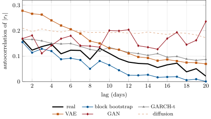
The table holds the chapter’s lessons. The scorecard is the weakest test: the VAE passes all six facts and is told apart from real windows 62% of the time; the block bootstrap passes all six and is indistinguishable (0.491) because its windows are pieces of real ones. The two-sample test sees what the scorecard misses, but not what matters for a strategy. Only TSTR measures that: the real model earns 0.86; the bootstrap’s windows keep most of the momentum inside their 20-day blocks (0.71); the VAE learned a noisy version of it (0.76, with a standard deviation of 0.28 across samples); GARCH, which cannot represent it, teaches nothing ($-0.10$, standard deviation 0.65: pure noise); the diffusion model teaches little (0.23).

16.5 The ways synthetic data mislead

Figure 16.2 is the hook’s result. On the GAN’s own windows a strategy earns a Sharpe ratio of 10.7: the generator produces far more linear autocorrelation (0.099 at lag 1, against 0.078 in the real windows) and persistent volatility patterns that a linear model can trade, an artefact of a network that has collapsed onto a few smooth shapes. Tested on real data, the same strategy earns 0.52. Every generator except GARCH shows a gap between TSTS and TSTR, and nothing inside the synthetic world reveals it.

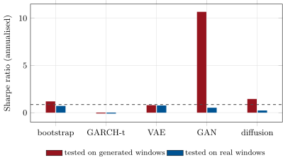
The memorisation column shows the other two failures. The block bootstrap’s windows are closer to a training window than the real test windows are three times as often as chance (14.5% against 5%): they are copies by construction, which is fine for stress tests and useless where synthetic data must protect the real data’s owner. The GAN’s 11.2% has a different cause: its windows are all calm, and calm windows have close neighbours among the many calm training windows. Nearest-neighbour distance flags copying and collapse alike, and has to be read with the tails. The memorisation of chapter 14 applies to generators as to language models: a large generator trained long enough on a small market history reproduces it.

Method 16.6 (Using synthetic market data)

1. Name the purpose (stress, training, testing a backtester, sharing), and choose the tests it needs.
2. Start from the classical generators (bootstrap, GARCH, a simulator with known mechanisms) and require a network to beat them on those tests.
3. Judge by TSTR against train-on-real, never by results inside the synthetic world; add the two-sample test with a blocked split and the memorisation check.
4. Treat any edge found only in synthetic data as an artefact until it is found in real data.

16.6 Tutorial: paths that never happened

16.7 Build: generators and their judges

16.8 Exercises

Exercise 16.1 ★

A two-sample test scores 0.62 on 4 000 generated against 4 000 real windows (2 000 of each held out). Is the difference from 0.5 significant? What would 0.51 tell you?

Solution

Solution of Exercise 16.1.

Under the null the held-out accuracy on 4 000 windows has standard error $\sqrt{0.25/4\,000} = 0.0079$: 0.62 is 15 standard errors above 0.5, a clear difference. 0.51 is 1.3 standard errors: no evidence of a difference, which is not evidence of equality; a stronger classifier or more samples might find one.

Exercise 16.2 ★

Which of the six stylised facts can a GARCH(1,1) model with symmetric Student-t shocks never produce, and why?

Solution

Solution of Exercise 16.2.

The leverage effect and gain-loss asymmetry: with symmetric shocks and a variance that responds to squared shocks, negative and positive returns raise volatility equally and the distribution of returns is symmetric. A GJR or EGARCH term and skewed shocks add them.

Exercise 16.3 ★

The fitted GARCH has $\alpha + \beta = 0.964$. What is the half-life of a volatility shock in days?

Solution

Solution of Exercise 16.3.

A shock to the variance decays like $(\alpha + \beta)^k$; the half-life is $\ln 0.5/\ln 0.964 = 19.1$ days.

Exercise 16.4 ★★

Why does the block bootstrap keep the momentum effect partly, and what block length would destroy it?

Solution

Solution of Exercise 16.4.

The effect links a day’s return to the previous twenty days’ sum; inside a 20-day block the ordering of real days is kept, so a window’s last day and its preceding days are often from the same block, and the relation survives there. Across block boundaries it is broken. Blocks of a few days destroy it; blocks much longer than twenty days keep it almost intact, and copy more of the history.

Exercise 16.5 ★★

Why did a random split make the two-sample test score real windows against real windows at 0.83?

Solution

Solution of Exercise 16.5.

Neighbouring windows share 31 of their 32 days. With a random split, almost every held-out window has a near-copy in the training half with the same label, so the classifier recognises the period, not the distribution: 0.83 for two halves of the same process. Splitting by year leaves no neighbours across the split.

Exercise 16.6 ★★

Find the flaw. “Our GAN’s paths pass all our stylised-fact tests, and a strategy trained on a million of them has a Sharpe ratio of 3 out of sample on another million, so it is robust.”

Solution

Solution of Exercise 16.6.

The test is inside the GAN’s world: a strategy trained and tested on generated paths measures the generator’s regularities, including artefacts. Here a GAN gives 10.7 inside its world and 0.52 on real data. Passing stylised-fact tests says nothing about predictability. Test the strategy on real data it was not trained on, and compare with training on real.

Exercise 16.7 ★★★

Coding. Train the GAN for 1 000 and for 8 000 steps. Report its excess kurtosis, two-sample accuracy and TSTS Sharpe ratio each time. Does longer training cure the collapse?

Solution

Solution of Exercise 16.7.

After 1 000 steps: excess kurtosis 2.53, two-sample accuracy 0.884, TSTS Sharpe ratio 11.2. After 8 000: 2.49, 0.734 and 9.9 (4 000 steps gave 1.98, 0.749 and 10.7). Longer training makes the windows harder to tell apart on average but does not restore the tails, which a discriminator on standardised windows rarely sees, and the invented predictability stays. The cures are architectural (heavy-tailed noise, a volatility channel as in Quant GANs) or a likelihood-based model.

Exercise 16.8 ★★★

Derive the VAE’s objective: show that $\log p(x)\ge\E_{q(z\mid x)}[\log p(x\mid z)] - \mathrm{KL}(q(z\mid x)\,\|\,p(z))$, and write the KL term for a diagonal Gaussian $q$ and a standard normal prior.

Solution

Solution of Exercise 16.8.

$\log p(x) = \log\int p(x\mid z)p(z)\,dz = \log\E_q[p(x\mid z)p(z)/q(z\mid x)]\ge\E_q[\log p(x\mid z)] + \E_q[\log p(z) - \log q(z\mid x)]$ by Jensen’s inequality, and the second term is $-\mathrm{KL}(q\,\|\,p)$. For $q = N(m, \mathrm{diag}\, s^2)$ and $p = N(0, I)$: $\mathrm{KL} = \tfrac12\sum_j(m_j^2 + s_j^2 - 1 - \log s_j^2)$, the term in the code.

16.9 Problem: Paths That Never Happened

Problem 16.1

Weekend problem — shape is not predictability

The chapter’s thirty years of returns, five generators and four tests.

Part I — The data and the generators.

1. What structure does the real series have, and which parts can each generator represent?
2. What are the fitted GARCH parameters, and what does the model miss?
3. What do the VAE and GAN networks look like, and how long do they train?
4. What is the diffusion model’s generating process?

Part II — Judging.

5. How many stylised facts does each generator pass?
6. What are the two-sample accuracies, and why must real windows be split by time?
7. What are the TSTR information coefficients and Sharpe ratios against train-on-real?
8. What does the memorisation check show?

Part III — Misleading.

9. What Sharpe ratio does the GAN’s world give, and where does it come from?
10. Why is GARCH’s TSTR noise, and how large is that noise?
11. Which generator would you use for a stress test, and which to augment a training set?
12. Why is the bootstrap unsuitable for sharing data outside the firm?

Part IV — The verdict.

13. State the named result: each generator’s scorecard pass count and two-sample accuracy, and the TSTR gap in Sharpe ratio.
14. What would convince you that a generator has learned a real predictability?
15. How would you test a backtester with a generator?
16. When is a mechanistic simulator better than a learned generator?
17. How would you condition a generator on a regime, and what new risk does it bring?
18. What would you log about a synthetic dataset used in research?
19. What does the diffusion model’s weakness at the tails imply for stress tests?
20. In one sentence: what does a generative model learn from twenty years of returns?

Solution

Solution of Problem 16.1.

Part I.

1. Fat tails, volatility clustering, a leverage effect, six crashes and a 20-day momentum effect. The bootstrap keeps what fits in a block; GARCH-t keeps tails and clustering; the networks can represent any of it in principle.
2. $\alpha = 0.079$, $\beta = 0.886$, 3.6 degrees of freedom; it misses the leverage effect, the skew and the momentum.
3. Multilayer perceptrons on standardised 32-day windows: a VAE with a four-dimensional code and a GAN with 16-dimensional noise and two layers of 128 units, 4 000 Adam steps each on one core.
4. Start from Gaussian noise and apply 100 learned denoising steps, each removing the predicted noise and adding a little fresh noise.

Part II.

1. Bootstrap 6, GARCH-t 4, VAE 6, GAN 3, diffusion 4 (real 6).
2. 0.491, 0.539, 0.619, 0.749, 0.693 (real against real 0.545). Overlapping windows leak across a random split: 0.83 for real against real.
3. IC and Sharpe: real 0.078 and 0.86; bootstrap 0.062 and 0.71; GARCH-t $-0.019$ and $-0.10$; VAE 0.040 and 0.76; GAN 0.052 and 0.52; diffusion 0.030 and 0.23.
4. Bootstrap windows are close to training windows 14.5% of the time (copies), GAN windows 11.2% (collapse onto calm windows), the others near the 5% of real test windows.

Part III.

1. 10.7, from linear autocorrelation and smooth volatility patterns the GAN invented.
2. GARCH-t has no predictability, so the fitted forecast is a random combination of features whose real-data IC is random in sign: $-0.10$ on average with a standard deviation of 0.65 across five samples.
3. A stress test needs tails and clustering: bootstrap or GARCH-t, with the crashes; augmentation needs the predictability without artefacts: none of the networks here is good enough, and the bootstrap’s copies add little new.
4. It reproduces real 20-day sequences: anyone with the real data can recognise them.

Part IV.

1. Paths that never happened. Facts passed and two-sample accuracy: bootstrap 6 and 0.491, GARCH-t 4 and 0.539, VAE 6 and 0.619, GAN 3 and 0.749, diffusion 4 and 0.693. TSTR Sharpe against 0.86 trained on real: 0.71, $-0.10$, 0.76, 0.52 and 0.23; the GAN’s own world gives 10.7.
2. TSTR close to train-on-real across several samples and fits, on a test period after the training data.
3. Plant known effects in generated data, run the backtester, and check that it recovers them and nothing else.
4. When the mechanism is the question (market impact, queue dynamics, a policy change), and when data are too few to learn a distribution.
5. Feed the regime as an input to the generator; the new risk is regimes that are rare in training and poorly generated exactly where stress tests need them.
6. The generator’s version and training data window, its seeds, the tests it passed, its purpose, and which results used it.
7. Tail losses from diffusion samples would be understated; stress with the tails from the real data or a heavy-tailed model.
8. Its shape, and only as much of its predictability as the architecture and the data force it to learn.

16.10 Interview questions

Interview question 16.1 ★ researcher, mle

Name the main stylised facts of daily returns. Which does a GARCH model reproduce?

Solution

Solution of Interview question 16.1.

Heavy tails, no linear autocorrelation, volatility clustering, the leverage effect, gain-loss asymmetry, aggregational Gaussianity, among others. GARCH with fat-tailed shocks reproduces tails, clustering and aggregation; asymmetric variants add leverage.

What the interviewer is looking for: four or more facts, and which a GARCH reproduces.

Interview question 16.2 ★★ mle

Explain the difference between a VAE, a GAN and a diffusion model in one paragraph each, and one failure of each.

Solution

Solution of Interview question 16.2.

VAE: an encoder to a latent distribution and a decoder, trained on a likelihood bound; samples are blurry or too Gaussian. GAN: a generator trained against a discriminator; mode collapse and unstable training. Diffusion: learned denoising of gradually noised data; slow sampling, and tails depend on training. Each fails differently on fat-tailed data.

What the interviewer is looking for: the training principle and a failure for each.

Interview question 16.3 ★★ researcher

How would you evaluate a generator of synthetic market data?

Solution

Solution of Interview question 16.3.

By purpose: stylised facts, a two-sample test with a time-blocked split, TSTR against train-on-real on later data, and a memorisation check; never by results inside the synthetic data alone.

What the interviewer is looking for: TSTR and a blocked two-sample test, tied to the purpose.

Interview question 16.4 ★★ researcher, trader

A colleague augments the training set with GAN paths and the backtest improves. What do you check?

Solution

Solution of Interview question 16.4.

Whether the improvement holds on real data not used to fit the generator; whether the generator was trained on the test period; whether synthetic paths carry artefacts the model learned (TSTS against TSTR); and whether the same effect appears with a bootstrap.

What the interviewer is looking for: real out-of-sample evaluation and generator leakage.

Interview question 16.5 ★★ mle

What is mode collapse, and how would you detect it in generated returns?

Solution

Solution of Interview question 16.5.

The generator covers only part of the distribution. Signs in returns: thin tails, too little diversity in volatility levels, generated windows close to a few typical real ones, a two-sample classifier winning on tail features.

What the interviewer is looking for: the definition and concrete diagnostics.

Interview question 16.6 ★★★ researcher

Design a classifier two-sample test for overlapping windows of a time series. What goes wrong with a random split?

Solution

Solution of Interview question 16.6.

Build features per window, split real windows by time blocks (with a gap longer than the window) so that no held-out window overlaps a training one, split generated windows at random, train, report held-out accuracy with its standard error. A random split puts near-copies on both sides and measures recognition of periods.

What the interviewer is looking for: blocked splitting with a gap, and why overlap inflates accuracy.