Machine Learning for Markets · Machine learning

5Trees and Boosting

The firm’s default gradient-boosted trees (300 trees of fifteen leaves) are fitted to ten years of a 300-stock panel and score $-0.19\%$ out of sample. A random search of twenty configurations finds one that scores 0.39% on the validation months and 0.32% on the test: four leaves, 200 slow trees. The search worked, for once. But rerun with four different random seeds, the defaults’ validation score ranges from 0.00% to 0.17%, and a search that compared the candidates against one draw of the defaults could have called anything between the two a success. Gradient boosting is the workhorse of the field on tabular data; this chapter builds it from trees, measures how it overfits on market data, and tunes it with the noise in view.

5.1 Trees

Definition 5.1 (Decision tree)

A decision tree partitions the feature space by a sequence of binary splits $x_j\le c$ , chosen greedily to reduce the loss most (for regression, the sum of squared errors), and predicts in each final cell, or leaf, the mean target of its training rows. Its capacity is set by its depth and by the minimum number of rows per leaf.

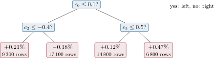
**Figure 5.1.** A tree of depth two on ranked characteristics, as a schematic: each split sends a stock-month left or right, each leaf predicts the mean demeaned return of its training rows. The leaf values and counts are illustrative, not fitted.

A tree captures interactions without being told (the right branch of Figure 5.1 lets characteristic 3 matter only when characteristic 0 is high) and does not care about monotone transformations of the features. Its weakness is variance: the split points and the leaf means are fitted to noise. On the chapter’s panel (300 stocks, 40 ranked characteristics with factor risk, 160 training months, a ceiling of 0.77% on the 80 test months) a tree of depth two scores 0.24% out of sample, depth five $-0.20\%$ , depth ten $-3.42\%$ .

5.2 Bagging and random forests

Definition 5.2 (Bagging, random forest, out-of-bag error)

Bagging (bootstrap aggregation) averages models fitted to bootstrap samples of the training set. A random forest bags deep trees and, at each split, considers only a random subset of the features, to decorrelate the trees. The out-of-bag error scores each training row with the trees whose bootstrap sample did not contain it.

Proposition 5.3 (What averaging buys)

If $B$ predictions have the same variance $\sigma^2$ and pairwise correlation $\rho$ , their average has variance $\rho\sigma^2 + (1 - \rho)\sigma^2/B$ .

Proof. $\Var(\frac1B\sum_bf_b) = \frac1{B^2}(B\sigma^2 + B(B-1)\rho\sigma^2) = \rho\sigma^2 + (1-\rho)\sigma^2/B$ . ∎

More trees remove only the second term; the first is removed by making the trees less correlated, which is what the random feature subsets are for. A forest of 40 trees (30% of the features per split, 300 rows per leaf) scores 0.20% on the test months. Its out-of-bag R-squared is 0.42%, twice as good, and its in-sample one 2.76%. The out-of-bag rows are not out of sample on a panel: each shares its month, and so its factor returns, with hundreds of in-bag rows that have similar characteristics. It is chapter 2’s warning about out-of-bag scores, in another guise.

5.3 Gradient boosting

Definition 5.4 (Gradient boosting, learning rate)

Gradient boosting builds an additive model $F_M(x) = F_0 + \eta\sum_{m=1}^Mh_m(x)$ one tree at a time: tree $h_m$ is fitted to the negative gradient of the loss with respect to the current predictions, $-\partial\ell(y_i, F_{m-1}(x_i))/\partial F$ , and added with a factor $\eta\in(0,1]$ . The learning rate $\eta$ is the step multiplier of an iterative fit: here the shrinkage of each tree, in gradient descent the size of each step (Book 4, chapter 24). Following the ML convention, $\eta$ denotes it in this book as a local symbol.

Proposition 5.5 (Boosting as gradient descent in function space)

For the squared loss $\ell(y, F) = \frac12(y - F)^2$ the negative gradient is the residual $y_i - F_{m-1}(x_i)$ , so each tree fits the current residuals. For any differentiable loss, one step $F_m = F_{m-1} + \eta h_m$ with $h_m$ equal to the negative gradient at the training points decreases the empirical loss for small enough $\eta$ .

Proof. $\partial\frac12(y - F)^2/\partial F = -(y - F)$ . For the second claim, $\mathcal L_n(F_{m-1} + \eta h) = \mathcal L_n(F_{m-1}) - \eta\frac1n\sum_ig_i^2 + O(\eta^2)$ with $g_i$ the gradient at row $i$ , when $h = -g$ at the training points; a tree approximates $-g$ and the same expansion holds with $\sum_ig_ih(x_i) < 0$ . ∎

The Huber loss of Book 4 (chapter 15) is the usual choice when returns have fat tails; LightGBM’s histogram-based trees, grown leaf by leaf, make the method fast enough to fit hundreds of models a day (Ke et al.).

5.4 Regularisation, early stopping and monotonic constraints

Definition 5.6 (Early stopping)

Early stopping stops an iterative fit (more trees, more epochs) at the iteration where the loss on a validation block, purged from the training rows, is lowest.

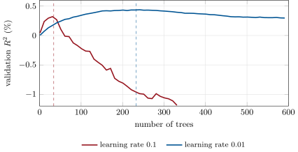
The number of trees and the learning rate trade against each other (Figure 5.2). At $\eta = 0.1$ the validation R-squared peaks after 34 trees and collapses afterwards; the stopped model scores 0.05% on the test months, the model run to 600 trees $-3.38\%$ . At $\eta = 0.01$ the peak comes after 233 trees and is higher and flatter; the stopped model scores 0.26% on the test months, and running to 600 trees costs little ( $0.03\%$ ). A small learning rate is a regulariser in its own right: each tree moves the fit so little that noise must be fitted slowly.

Validation R-squared (40 purged months) of boosted trees as trees are added, at two learning rates; dashed, the early-stopping points (34 and 233 trees). The curve at = 0.1 leaves the frame after about 340 trees and reaches -2.9\% at 600. Data: ml_trees.early. — **Figure 5.2.** Validation R-squared (40 purged months) of boosted trees as trees are added, at two learning rates; dashed, the early-stopping points (34 and 233 trees). The curve at $\eta = 0.1$ leaves the frame after about 340 trees and reaches $-2.9\%$ at 600. Data: `ml_trees.early`.

Definition 5.7 (Monotonic constraint)

A monotonic constraint restricts a model to be non-decreasing (or non-increasing) in a feature, all others fixed. In a tree ensemble it is enforced by allowing a split on that feature only when the left child’s value does not exceed the right child’s (or the reverse), propagated down the tree.

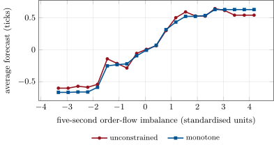
Microstructure often knows a sign the data are too noisy to show. On firm.tape sessions a larger order-flow imbalance should never forecast a lower mid price (Book 7, chapter 8). Boosted trees fitted to five-second mid changes on eight ten-minute sessions (912 non-overlapping labels, ten order-book features) and tested on eight more score an R-squared of 0.333 unconstrained, 0.364 with the seven imbalance and flow features constrained to act positively. Unconstrained, a push of half a standard deviation in the five-second imbalance lowers the forecast for 7.0% of the test rows; with the constraints, for none (Figure 5.3). The constraint is prior knowledge used as regularisation, and it is also a guarantee a risk committee can read. (The R-squared are high because the simulated mid trends over a few seconds, a property of firm.tape Book 7 documents; the comparison is the point, not the level.)

Partial dependence of the five-second forecast on the order-flow imbalance (the feature swept over its 2nd to 98th percentile, the others at their observed values), for boosted trees without and with monotonic constraints. Data: ml_trees.partial_dependence on firm.tape. — **Figure 5.3.** Partial dependence of the five-second forecast on the order-flow imbalance (the feature swept over its 2nd to 98th percentile, the others at their observed values), for boosted trees without and with monotonic constraints. Data: `ml_trees.partial_dependence` on `firm.tape`.

5.5 Tuning under noise

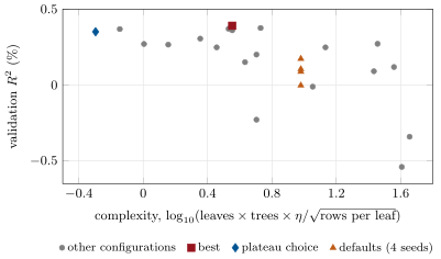
A random search draws twenty configurations (leaves, learning rate, trees, rows per leaf, row and column sampling, an $\ell_2$ penalty) and scores each on the validation block (Figure 5.4). Their validation R-squared ranges from $-0.54\%$ to 0.39%. The winner has four leaves, a learning rate of 0.02 and 200 trees; retrained with four seeds it scores 0.36–0.39% (a standard deviation of 0.014 points), and 0.32% on the test months, 0.07 points below its validation score, as chapter 3 predicts for a winner. The defaults, retrained with the same four seeds, score between 0.00% and 0.17% (a standard deviation of 0.07 points) and $-0.19\%$ on the test months.

Two lessons come out of it. Complex configurations are noisy as well as bad: the seed-to-seed spread of the defaults is five times that of the winner, so a single validation run of a complex model is a poor estimate of it, and a search that rescores its top candidates with several seeds is cheap insurance. And the good region is a plateau: six of the twenty configurations sit within 0.04 points of the best. Choosing the least complex configuration within one seed standard deviation of the best (four leaves, 1 000 rows per leaf, no subsampling) gives 0.35% on validation and 0.31% on test, as good, with a model a seventh as flexible by the measure of Figure 5.4.

Twenty random configurations of boosted trees on the validation months, against a crude measure of their flexibility; the defaults retrained with four seeds. Data: ml_trees.tuning. — **Figure 5.4.** Twenty random configurations of boosted trees on the validation months, against a crude measure of their flexibility; the defaults retrained with four seeds. Data: `ml_trees.tuning`.

Method 5.8 (Tuning boosted trees on market data)

Fix a purged validation block (or purged folds) and never tune on the test.
Start from a small learning rate (0.01–0.03) with early stopping, few leaves and many rows per leaf.
Search randomly over the regularisers; rescore the top few candidates with several seeds.
Choose from the plateau (the least flexible within one seed standard deviation of the best), not the peak.
Declare monotonic constraints wherever the economics fixes a sign.

5.6 Tutorial: tuning in the fog

Goal. Fit trees, a forest and boosted trees to the panel; stop boosting early at two learning rates; run a random search and choose from its plateau; constrain order-book features on firm.tape. End state: the chapter’s numbers and Figures 5.2, 5.3 and 5.4.

Early stopping through LightGBM’s callbacks, keeping the validation curve.

def fit_early_stop(params, X, y, Xv, yv, max_trees: int = 1000, patience: int = 50, monotone=None, names=None,
                   seed: int = 1):
    """Fit up to max_trees and keep the number of trees with the best validation loss; `curve` is the validation MSE
    after each tree. The validation block must be purged from the training rows by the caller."""
    import lightgbm as lgb

    m = make(dict(params or {}, n_estimators=max_trees), monotone, names, seed)
    m.fit(X, y, eval_X=(Xv,), eval_y=(yv,), eval_metric="l2",
          callbacks=[lgb.early_stopping(patience, verbose=False), lgb.record_evaluation(rec := {})])
    curve = np.asarray(rec["valid_0"]["l2"])
    return m, int(m.best_iteration_), curve

Listing 5.1. Early stopping on a purged validation block. code/firm/gbdt/firm_gbdt.py

The plateau rule and the model dump: the fitted trees become a dictionary that a NumPy function evaluates exactly (chapter 26 compiles the same dictionary).

def plateau_select(scores, se: float, complexity) -> int:
    """Among candidates whose score is within `se` of the best, the one with the lowest complexity."""
    scores, complexity = np.asarray(scores, float), np.asarray(complexity, float)
    ok = np.flatnonzero(scores >= scores.max() - se)
    return int(ok[np.argmin(complexity[ok])])


def to_dict(model) -> dict:
    return model.booster_.dump_model()


def _eval_tree(node, X, out, idx):
    if "leaf_value" in node:
        out[idx] += node["leaf_value"]
        return
    f, thr, mt = node["split_feature"], node["threshold"], node.get("missing_type", "None")
    x = X[idx, f]
    miss = np.isnan(x)
    if mt == "NaN":                                                     # learned direction for missing values
        left = np.where(miss, node["default_left"], x <= thr)
    elif mt == "Zero":                                                  # zeros (and NaN) follow the default side
        z = miss | (x == 0.0)
        left = np.where(z, node["default_left"], x <= thr)
    else:                                                               # no missing values in training: NaN -> 0
        left = np.where(miss, 0.0, x) <= thr
    _eval_tree(node["left_child"], X, out, idx[left])
    _eval_tree(node["right_child"], X, out, idx[~left])


def predict_dict(d: dict, X) -> np.ndarray:
    """Sum of the trees' leaf values (LightGBM stores the initial score inside the first tree's leaves)."""
    X = np.asarray(X, float)
    out = np.zeros(len(X))
    for t in d["tree_info"]:
        _eval_tree(t["tree_structure"], X, out, np.arange(len(X)))
    return out

Listing 5.2. Choosing from the plateau; evaluating dumped trees. code/firm/gbdt/firm_gbdt.py

Run ml_trees.family(), early(), tuning(), monotone() and fig_trees.py.

What to change next. Constrain the order-flow imbalance with the wrong sign and measure the cost; rescore every configuration of the search with four seeds and see whether the winner changes.

5.7 Build: the firm’s boosted trees

Purpose. One way to fit, stop, constrain, ensemble, choose and export gradient-boosted trees.

Interface. make(params, monotone, names, seed), DEFAULTS, fit_early_stop(params, X, y, Xv, yv, max_trees, patience, monotone, names, seed), SeedEnsemble(params, seeds, monotone, names), plateau_select(scores, se, complexity), to_dict(model), predict_dict(d, X).

Rules. Deterministic, single-threaded fits; the validation block is purged by the caller; constraints are declared by feature name, never by column position; exported dictionaries reproduce predictions exactly, missing values included.

Acceptance tests. code/firm/gbdt/tests/: two fits give identical predictions; the dictionary evaluator matches LightGBM with missing values; early stopping keeps the best iteration and the dump holds only it; a monotone feature never lowers the prediction; seed ensembles average; the plateau rule picks the simplest near-best candidate.

Stretch. Quantile and Huber losses through the same interface; a warm-started refit that adds trees for new months (chapter 12).

Sources and further reading

L. Breiman, “Random forests”, Machine Learning 45, 2001.
J. H. Friedman, “Greedy function approximation: a gradient boosting machine”, Annals of Statistics 29(5), 2001.
G. Ke et al., “LightGBM: a highly efficient gradient boosting decision tree”, Advances in Neural Information Processing Systems 30, 2017.
T. Chen and C. Guestrin, “XGBoost: a scalable tree boosting system”, KDD, 2016.
L. Grinsztajn, E. Oyallon and G. Varoquaux, “Why do tree-based models still outperform deep learning on typical tabular data?”, NeurIPS Datasets and Benchmarks, 2022.

5.8 Exercises

Exercise 5.1 ★

Fifty trees each have prediction variance $\sigma^2$ and pairwise correlation 0.3. What is the variance of their average? And with infinitely many trees?

Solution

Solution of Exercise 5.1.

$0.3\sigma^2 + 0.7\sigma^2/50 = 0.314\sigma^2$ ; with infinitely many trees, $0.3\sigma^2$ : only decorrelation lowers the floor.

Exercise 5.2 ★

A tree splits 1 000 rows into two leaves of 400 and 600 rows whose mean targets are $-0.1$ and $+0.2$ . The overall mean is $0.08$ . By how much does the split reduce the sum of squared errors?

Solution

Solution of Exercise 5.2.

$400\times(-0.1 - 0.08)^2 + 600\times(0.2 - 0.08)^2 = 12.96 + 8.64 = 21.6$ .

Exercise 5.3 ★

Boosting with squared loss starts from $F_0 = 0$ ; a row has target 1.0 and the first tree predicts 0.8 for it. With $\eta = 0.1$ , what is the row’s residual after the first step? What would it be after ten steps if every tree, the first included, predicted its current residual exactly?

Solution

Solution of Exercise 5.3.

$F_1 = 0.1\times0.8 = 0.08$ , residual 0.92. If each tree predicted the current residual exactly, each step would keep $1 - \eta = 0.9$ of it: $0.9^{10} = 0.349$ after ten steps.

Exercise 5.4 ★★

Why is the forest’s out-of-bag R-squared (0.42%) twice its test R-squared (0.20%) on the panel?

Solution

Solution of Exercise 5.4.

An out-of-bag row shares its month, hence its factor returns, with hundreds of in-bag rows of similar characteristics; the trees have learned that month’s factor moves from them, so the row is not out of sample. The test months share nothing with the training months.

Exercise 5.5 ★★

The defaults’ validation score over four seeds is 0.17, 0.11, 0.09 and 0.00%. A candidate scores 0.14% on one seed. Is it better than the defaults? What would you do before deciding?

Solution

Solution of Exercise 5.5.

The defaults average 0.09% with a standard deviation of 0.07 points across seeds; 0.14% on one seed is within one standard deviation of their mean. Rescore the candidate with the same four seeds (and on purged folds) before calling it better.

Exercise 5.6 ★★

Find the flaw. “We used early stopping on the test months to pick the number of trees, and report the test R-squared at that point.”

Solution

Solution of Exercise 5.6.

The number of trees was chosen on the test months, so the test score is a selection score, optimistic by Proposition 3.2. Stop on a validation block purged from both the training and the test months.

Exercise 5.7 ★★★

Coding. In ml_trees.monotone, constrain the five-second order-flow imbalance to act negatively (all other constraints as in the chapter). Report the test R-squared and explain the result.

Solution

Solution of Exercise 5.7.

monotone(ofi5_sign=-1): R-squared 0.305, against 0.333 unconstrained and 0.364 with the right sign; raising the imbalance now lowers the forecast for 95% of the rows. A wrong constraint is a wrong prior imposed exactly; it costs more than no constraint.

Exercise 5.8 ★★★

Show that with squared loss and a learning rate $\eta$ , if every tree fitted the residuals exactly, a row’s residual after $M$ trees would be $(1 - \eta)^M$ times its target; explain why this makes early stopping and a small learning rate substitutes.

Solution

Solution of Exercise 5.8.

With squared loss and exact fits, $F_m = F_{m-1} + \eta(y - F_{m-1})$ , so $y - F_m = (1 - \eta)(y - F_{m-1})$ and, from $F_0 = 0$ , $y - F_M = (1 - \eta)^My$ . The fit’s progress depends on $\eta M$ roughly (for small $\eta$ , $(1 - \eta)^M \approx e^{-\eta M}$ ): halving the learning rate doubles the trees needed, and stopping early at a given $\eta$ is like choosing a smaller effective $\eta M$ . Real trees fit residuals only partly and fit noise too, which is why a small $\eta$ with more trees generalises better than a large one with few.

5.9 Problem: Tuning in the Fog

Problem 5.1

Weekend problem — twenty configurations and a plateau

The chapter’s panel: 300 stocks, forty characteristics with factor risk, 160 training months (the last 40 of them as a purged validation block when tuning), 80 test months.

Part I — Single trees and forests.

What do trees of depth 2, 5 and 10 score out of sample, and why the ordering?
What does the forest score out of sample, out of bag and in sample?
Why is the out-of-bag score optimistic on a panel?
What does Proposition 5.3 say more trees can and cannot do?

Part II — Boosting and early stopping.

What do the defaults score on the test months?
Where does early stopping stop at $\eta = 0.1$ and $0.01$ , and what do the stopped models score?
What would running to 600 trees have cost at each learning rate?
Why is a small learning rate a regulariser?

Part III — The search.

What range of validation scores do the twenty configurations cover?
What is the winner, and what does it score with four seeds and on the test months?
How noisy are the defaults across seeds compared with the winner?
Which configuration does the plateau rule choose, and what does it score?

Part IV — Constraints and the verdict.

What do monotonic constraints do to the order-book model’s R-squared and to its violations?
Why can a constraint improve an out-of-sample score?
State the named result: the seed standard deviation of the defaults’ and of the winner’s validation score against the gain from tuning, and the winner’s validation-to-test gap.
Which configuration would you put in production, and why?
How many seeds would you use to rescore the top candidates of a search?
What should the research log record about the search?
What would change with ten times more stocks?
In one sentence: how should boosted trees be tuned on market data?

Solution

Solution of Problem 5.1.

0.24%, $-0.20\%$ , $-3.42\%$ : deeper trees fit more noise (the variance term).
0.20% out of sample, 0.42% out of bag, 2.76% in sample.
Out-of-bag rows share their month’s factor returns with in-bag rows.
More trees remove the $(1-\rho)\sigma^2/B$ term; only less correlated trees lower $\rho\sigma^2$ .
$-0.19\%$ .
After 34 trees at 0.1 (test 0.05%) and 233 trees at 0.01 (test 0.26%).
At 0.1, the test R-squared falls to $-3.38\%$ ; at 0.01, to 0.03%.
Each tree moves the fit a little, so noise must be fitted slowly and the validation curve is flat near its peak.
From $-0.54\%$ to 0.39%.
Four leaves, learning rate 0.02, 200 trees, 20 rows per leaf; 0.36–0.39% with four seeds, 0.32% on the test.
Standard deviations of 0.07 points for the defaults, 0.014 for the winner: five times noisier.
Four leaves, 1 000 rows per leaf, no subsampling: 0.35% on validation, 0.31% on test.
R-squared 0.333 to 0.364; violations from 7.0% of the rows to none.
It removes directions of fit that only noise supports: a restriction that the truth satisfies lowers variance without adding bias.
Named result: the defaults’ validation score varies with the seed by 0.07 points (0.00–0.17%) and the winner’s by 0.014, against a gain from tuning of about 0.3 points (0.09% to 0.39%); the winner loses 0.07 points from validation to test.
The plateau choice: as good on test, less flexible, and less sensitive to the seed.
Three to five, enough to see a standard deviation; more if the candidates are within one of each other.
Every configuration and its score, the seeds, the validation block, and the rule used to choose.
The effective sample of the characteristics’ effects is the months, so more stocks help less than more months; complex configurations would still be noisy.
Small learning rates, few leaves, many rows per leaf, early stopping on purged data, several seeds, and a choice from the plateau.

5.10 Interview questions

Interview question 5.1 ★ researcher, mle

Explain the difference between bagging and boosting.

Solution

Solution of Interview question 5.1.

Bagging averages models fitted independently to bootstrap samples, reducing variance; boosting fits models in sequence, each to the errors of the ensemble so far, reducing bias (and, with shrinkage and early stopping, controlling variance).

What the interviewer is looking for: parallel versus sequential, variance versus bias.

Interview question 5.2 ★ mle

Which hyperparameters of a gradient-boosted model would you tune first on noisy data, and in which direction?

Solution

Solution of Interview question 5.2.

The ones that control variance: a small learning rate with early stopping, few leaves or shallow depth, a large minimum number of rows per leaf, row and column subsampling, an $\ell_2$ penalty. All in the direction of less flexibility.

What the interviewer is looking for: regularisers first, and the direction on low signal-to-noise data.

Interview question 5.3 ★★ researcher

Why might a random forest’s out-of-bag error be misleading on financial panel data?

Solution

Solution of Interview question 5.3.

Out-of-bag rows share dates (and common factor shocks, overlapping labels) with in-bag rows, so they are not independent test data; the score is optimistic. Use purged, time-ordered validation.

What the interviewer is looking for: the dependence between rows of a panel.

Interview question 5.4 ★★ researcher, trader

What is a monotonic constraint, and give two features of a trading model you would constrain.

Solution

Solution of Interview question 5.4.

A restriction that the model be non-decreasing (or non-increasing) in a feature. Candidates: order-flow imbalance and queue imbalance (a higher bid-side pressure should not predict a lower price); a borrow fee in a short-squeeze model; a distance to a price limit.

What the interviewer is looking for: the definition and economically justified signs.

Interview question 5.5 ★★ mle

Two boosting configurations differ by 0.03 points of validation R-squared. How do you decide between them?

Solution

Solution of Interview question 5.5.

Compare with the noise first: rescore both with several seeds and on purged folds; if they are within one standard deviation, take the simpler, less turnover-prone, or better-constrained one.

What the interviewer is looking for: noise before ranking, then simplicity.

Interview question 5.6 ★★★ researcher, mle

Derive why boosting with squared loss fits residuals, and what changes with a Huber loss.

Solution

Solution of Interview question 5.6.

The negative gradient of $\frac12(y - F)^2$ in $F$ is $y - F$ , the residual, so each tree fits residuals. With the Huber loss the gradient is the residual clipped at $\pm\delta$ : large errors (fat-tailed returns) pull the fit less.

What the interviewer is looking for: the gradient computation and the robustness of the Huber loss.

Terms defined in this chapter

See all 2333 terms in the glossary