2Targets, Labels and Sample Weights

A classifier is trained to say whether an asset will be up ten days from now, and it does so a little better than a coin. The trader who will use it asks what it does about the stop-loss: every position is closed if it loses one ten-day volatility, and taken profit if it gains one. On twenty synthetic assets over ten years, one trade in five hits its stop before day ten; the label the classifier learned never saw the stop. And the training set that looked like 49 000 examples holds, once the overlap of ten-day windows is counted, the information of 4 900. This chapter builds labels that describe the trade, measures how much labels overlap, and turns the overlap into sample weights and honest statistics.

2.1 Fixed-horizon labels and their flaws

The data of the chapter come from firm.mlsynth.series: twenty assets, 2 520 days, daily volatility 1.5% with GARCH clustering and Student-$t$ shocks, and a planted drift, persistent with a half-life of 20 days, whose correlation with the next day’s return is 0.04. The features, known at each close, are a noisy reading of the drift, the 5- and 20-day past returns, a ratio of short to long realised volatility and three pure-noise columns. An event is every day of every asset; the primary trade is long when the drift reading is positive and short otherwise.

Definition 2.1 (Fixed-horizon label)

Given an event at bar $t_0$ and a horizon $h$, the fixed-horizon label is $\sign(\sum_{s=t_0+1}^{t_0+h}R_s)$, or the return itself for regression, settled at $t_1 = t_0 + h$.

The fixed-horizon label is Book 7’s forward return (chapter 6) turned into a class. It has three flaws. It ignores the path: a position that would have been stopped out on day three and a position that ended up on day ten get the same label if the price came back. It ignores the volatility: a 1% move is noise on a volatile day and news on a quiet one. And it ends at a fixed time, so the labels of consecutive events overlap in $h - 1$ of their $h$ bars. The first two are fixed by the barrier label below; the third by counting (Section 2.3).

2.2 Barrier labels and meta-labelling

Definition 2.2 (Triple-barrier label)

For an event at $t_0$ with position side $\pm1$, widths $w^+, w^- > 0$ and a horizon $h$, the triple-barrier label settles at the first bar $t_1$ at which the position’s cumulative log return reaches $+w^+$ (profit-taking), $-w^-$ (stop-loss), or $t_1 = t_0 + h$ (the vertical barrier); it is the sign of the position’s return at $t_1$. The widths are usually scaled by the volatility known at $t_0$: $w = k\hat\sigma_{t_0}\sqrt h$ (López de Prado, 2018).

With $k = 1$ and $h = 10$, the long-or-short trade of the chapter hits its profit barrier first 22.7% of the time, its stop 20.3% of the time, and the vertical barrier otherwise; a label lasts 8.3 days on average instead of 10. Figure 2.1 shows one event of the first asset: a long position stopped on day three at $-5.04\%$ (the width was 4.87%), when the price went on to end day ten 1.84% higher. The fixed-horizon label calls that trade a winner. It is one case of many: of the trades stopped out, 5.3% end positive at day ten. Signs disagree for 1.9% of all events; what differs everywhere is the size, since the barrier label’s returns are truncated at the barriers as the trade’s are.

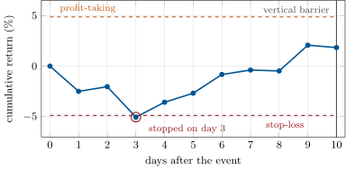
The side of a trade and its size are different questions. A primary model (a rule, a researcher’s signal, a discretionary call) may be good at the side and poor at knowing when it is right.

Definition 2.3 (Meta-labelling)

Meta-labelling labels each event of a primary model with 1 if the trade in the primary model’s direction made money (for example, its triple-barrier return is positive) and 0 otherwise, and trains a secondary model on these labels to estimate the probability that the primary call is right; the probability is then used to filter or size the trade (López de Prado, 2018; Joubert, 2022).

Meta-labelling the chapter’s trade with gradient-boosted trees (Figure 2.2), trained on the first 60% of the dates and scored on the last 40%, raises the hit rate of the trades it keeps from 53.0% to 54.5% and the average return per trade from 0.064 to 0.097 barrier widths when it keeps the third of the trades it is most confident about. The overlap-adjusted $t$-statistic falls from 3.48 to 3.19: the kept trades are better, and there are fewer of them. Meta-labelling reallocates risk to the better trades; it does not create a signal the primary model lacks.

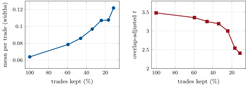
2.3 Overlap, concurrency and uniqueness

Definition 2.4 (Label concurrency, average uniqueness)

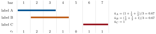
Label $i$ spans the bars $(t_{0,i}, t_{1,i}]$. The label concurrency $c_t$ of bar $t$ is the number of labels whose span contains it. The average uniqueness of label $i$ is $\bar u_i = \frac{1}{t_{1,i} - t_{0,i}}\sum_{t\in(t_{0,i}, t_{1,i}]}1/c_t$: the share of its information it holds alone.

Figure 2.3 is the smallest example: three labels over seven bars, two of them overlapping in two bars. Book 7 named the phenomenon (label overlap, chapter 20) and removed its leak from cross-validation by purging; here it is measured, because it changes how much the sample is worth.

Proposition 2.5 (How much overlapping labels are worth)

1. If every label spans $h$ bars, $\sum_i\bar u_i = N_{\mathrm{cov}}/h$, where $N_{\mathrm{cov}}$ is the number of bars covered by at least one label. With an event on every bar, $\bar u_i = 1/h$ away from the ends.
2. If returns are uncorrelated with variance $\sigma^2$ and the $n$ labels are the overlapping $h$-bar sums of one series, the sample mean of the labels has variance about $h^2\sigma^2/n$, $h$ times the $h\sigma^2/n$ that treating them as independent assumes: a $t$-statistic computed on $n$ rows is inflated by about $\sqrt h$.

On the chapter’s data the fixed-horizon labels have a concurrency of exactly 10 and an average uniqueness of 0.100: 48 980 labels are worth 4 916, as part 1 predicts ($20\times2\,458/10$). The barrier labels, shorter, have a uniqueness of 0.123 and are worth 6 040. The primary trade’s average return has a $t$-statistic of 9.4 computed on the rows and 3.3 with the number of trades replaced by the sum of uniqueness: the ratio, 2.85, is $\sqrt{1/0.123}$.

2.4 Sample weights and the sequential bootstrap

Definition 2.6 (Sample weight, time-decay weight)

A sample weight $\omega_i\ge0$ scales observation $i$’s term in the empirical loss, $\mathcal L_n(\theta) = \sum_i\omega_i\ell(y_i, f_\theta(x_i))/\sum_i\omega_i$. Three are common on market data: uniqueness weights $\omega_i = \bar u_i$; return-attribution weights, $\omega_i\propto|\sum_{t\in i}R_t/c_t|$, which favour labels whose moves they own; and a time-decay weight, which falls linearly from 1 for the newest label to a floor for the oldest, in units of cumulative uniqueness, so that old data count less.

Definition 2.7 (Sequential bootstrap)

The sequential bootstrap draws labels one at a time, with replacement, each with probability proportional to the average uniqueness it would have given the labels already drawn; overlapping labels become less likely once one of them is in the sample.

The case for these tools is that a bagged ensemble whose bootstrap samples are full of near-duplicates grows correlated trees, each fitted to the same few independent observations. Drawing 40 of the first 400 ten-day labels of one asset (about their effective number), the plain bootstrap’s samples have an average uniqueness of 0.65 and the sequential bootstrap’s 0.69. Whether it matters for prediction is an empirical question, and on this data the answer is no (Table 2.1): bagged trees trained on plain bootstrap samples, on samples as small as the average uniqueness times the sample size, and on those samples weighted by uniqueness have the same out-of-sample AUC in three simulated markets, within $\pm0.007$ of each other and in no consistent order. The trees were regularised (at least 50 labels per leaf, 5 in the small samples), and none of the features identifies a date, which is what lets near-duplicates leak in the first place. Where overlap does bite without fail is in every statistic that counts rows: standard errors, $t$-statistics, bootstrap intervals and out-of-bag scores.

bootstrap samples	market 1	market 2	market 3	mean
plain, full size	0.504	0.517	0.509	0.510
average-uniqueness size	0.511	0.512	0.506	0.510
same, weighted by uniqueness	0.506	0.511	0.510	0.509

Method 2.8 (Labels and weights for a new study)

1. Write the trade first (side, entry, exits, horizon), then the label that settles it: barriers at the trade’s stop and target, scaled by volatility known at the event.
2. Store every label with its $t_0$ and $t_1$; compute concurrency and uniqueness per asset.
3. Report the effective sample $\sum_i\bar u_i$ beside the number of rows, and compute every standard error with it (or with a block bootstrap of Book 4, chapter 13).
4. Try uniqueness and time-decay weights as hyperparameters, on validation folds that are purged (chapter 3); keep them only if they help there.

2.5 Tutorial: labels that describe the trade

2.6 Build: labels and sample weights

2.7 Exercises

Exercise 2.1 ★

Labels of 5 bars start on every bar of a 1 000-bar series (the last ones truncated at the end). About how many independent labels do they amount to, and what is their average uniqueness away from the ends?

Solution

Solution of Exercise 2.1.

About $1\,000/5 = 200$ independent labels (Proposition 2.5); uniqueness $1/5 = 0.2$ away from the ends.

Exercise 2.2 ★

Four labels span bars $(0,2]$, $(1,4]$, $(2,4]$ and $(6,8]$. Write the concurrency of bars 1 to 8 and each label’s average uniqueness.

Solution

Solution of Exercise 2.2.

Bars 1 to 8: $c = 1, 2, 2, 2, 0, 0, 1, 1$. Uniqueness: $(1 + \tfrac12)/2 = 0.75$; $(\tfrac12 + \tfrac12 + \tfrac12)/3 = 0.5$; $(\tfrac12 + \tfrac12)/2 = 0.5$; $1$.

Exercise 2.3 ★

The daily volatility known at an event is 1.2%. What are the barrier widths for $k = 1.5$ and a horizon of 16 days?

Solution

Solution of Exercise 2.3.

$1.5\times1.2\%\times\sqrt{16} = 7.2\%$ each side.

Exercise 2.4 ★★

A strategy’s average trade has a $t$-statistic of 6.1 computed on 25 000 overlapping 20-day trades opened every day. What $t$-statistic should be reported, and why?

Solution

Solution of Exercise 2.4.

Trades opened daily with 20-day spans have uniqueness about $1/20$, so the effective count is about 1 250 and the $t$-statistic about $6.1/\sqrt{20} = 1.36$: not significant.

Exercise 2.5 ★★

Why does meta-labelling raise the average return per trade but not the $t$-statistic of the whole book, in Figure 2.2? When would it raise both?

Solution

Solution of Exercise 2.5.

The $t$-statistic is the mean over the standard deviation times the square root of the effective number of trades. Keeping a third of the trades raises the mean by half (0.064 to 0.097 widths) but divides the effective count by about three, so $t$ falls (3.48 to 3.19). It would rise if the secondary model found trades with negative expectation to drop (information the primary model lacks), not merely trades with a smaller positive one.

Exercise 2.6 ★★

Find the flaw. “Our barrier widths are set at one standard deviation of each asset’s daily returns over the whole sample, times the square root of the horizon.”

Solution

Solution of Exercise 2.6.

The whole-sample standard deviation uses the future (look-ahead) and ignores volatility clustering: barriers are too wide in calm periods and too narrow in stress, so labels settle for reasons unrelated to the trade. Use the volatility known at the event (EWMA or GARCH, Book 4, chapter 18).

Exercise 2.7 ★★★

Coding. Rebuild ml_labels.events with barriers at two ten-day volatilities ($k = 2$). Report the shares of profit, stop and vertical exits and the average uniqueness of the barrier labels, and explain the change.

Solution

Solution of Exercise 2.7.

label_stats(k=2.0): profit 4.0%, stop 3.3%, vertical 92.7%; labels last 9.8 days, uniqueness 0.1025 (0.123 at $k = 1$). Wider barriers are rarely touched within ten days, so the barrier label converges to the fixed-horizon label.

Exercise 2.8 ★★★

With time-decay weights falling linearly from 1 to 0.5 in cumulative uniqueness, and every label of uniqueness 0.1, what is the weight of the label halfway through the sample? Show that the weights’ mean is 0.75 whatever the uniqueness if it is constant, and say what changes when it is not.

Solution

Solution of Exercise 2.8.

With constant uniqueness, cumulative uniqueness is proportional to the label’s rank: the halfway label has weight $0.5 + 0.5\times0.5 = 0.75$, and the average of a linear ramp from 0.5 to 1 is 0.75. With varying uniqueness, crowded periods (low uniqueness) advance the ramp slowly, so their many labels share similar weights and the decay follows information, not the calendar; the mean then depends on where the crowded periods fall.

2.8 Problem: Five Hundred Overlapping Days

Problem 2.1

Weekend problem — what a training set is worth

The chapter’s twenty assets, their daily events and the primary long-or-short trade.

Part I — Two labels.

1. How often does the trade hit its profit barrier, its stop, the vertical barrier?
2. How long does a barrier label last on average, and why is it shorter than ten days?
3. In Figure 2.1, what do the fixed-horizon and the barrier label say, and which describes the trade?
4. What share of all events have labels of opposite signs, and why is that not the whole difference?

Part II — Overlap.

5. What are the concurrency and the average uniqueness of the fixed-horizon labels?
6. How many independent labels are the 48 980 worth, by Proposition 2.5? And the barrier labels?
7. Give the trade’s $t$-statistic on rows and adjusted for overlap, and explain their ratio.
8. Which statistics of a study are wrong if overlap is ignored?

Part III — Weights and bootstraps.

9. What average uniqueness do plain and sequential bootstrap samples of 40 labels have?
10. What AUC do the three bagging schemes reach, market by market?
11. Why did uniqueness make no difference to the AUC here?
12. Design a setting where it would.

Part IV — Meta-labelling and the verdict.

13. What do the kept trades gain at a threshold of 0.52, and what does the book lose?
14. Why is meta-labelling sizing, not alpha?
15. Would you use the probability to size rather than to filter? How?
16. State the named result: the effective number of observations against the nominal one, the $t$-statistic before and after, and the AUC gain of uniqueness weighting over plain bagging with its spread.
17. What would the effective sample be with 20-day labels?
18. How should a research log record the size of a training set?
19. What does purging (Book 7) have to do with uniqueness?
20. In one sentence: what is a label?

Solution

Solution of Problem 2.1.

1. Profit 22.7%, stop 20.3%, vertical 57.0%.
2. 8.3 days: a label settles at the first touch, before day ten in 43% of the events.
3. Fixed horizon: up (a winner, $+1.84\%$); barrier: stopped at $-5.04\%$ on day three, a loser. The barrier label describes the trade.
4. 1.9%; sizes differ for every touched label, since barrier returns are truncated as the trade’s are.
5. Concurrency 10, uniqueness 0.100.
6. $20\times2\,458/10 = 4\,916$; barrier labels 6 040.
7. 9.4 on rows, 3.3 adjusted; ratio $2.85 = \sqrt{1/0.123}$ (Proposition 2.5, part 2).
8. Standard errors, $t$-statistics, bootstrap intervals, out-of-bag scores, and any significance test that counts rows.
9. 0.65 and 0.69.
10. Plain 0.504, 0.517, 0.509; small 0.511, 0.512, 0.506; weighted 0.506, 0.511, 0.510.
11. The trees were regularised and no feature identifies the date, so near-duplicates in a bootstrap sample could not be memorised into an advantage.
12. Deep trees with a slowly moving feature that locates time (a regime variable, a trend of the level): overlapping neighbours then share both features and labels, and full-size bootstrap samples fit them.
13. Hit rate 54.5% against 53.0% and 0.097 against 0.064 widths per trade, on a third of the trades; the overlap-adjusted $t$ falls from 3.48 to 3.19.
14. It chooses which of the primary model’s trades to take and how much; the side, where the signal is, comes from the primary model.
15. Yes, in proportion to $2p - 1$ or to a Kelly-like fraction (chapter 11), which keeps every trade but scales it: filtering is the special case of sizes 0 and 1.
16. Named result: 4 916 effective labels of 48 980 (10%); $t$ of 9.4 on rows, 3.3 adjusted; uniqueness weighting’s AUC gain over plain bagging $-0.001$ on average, within $\pm0.007$ market by market.
17. About $20\times2\,450/20 = 2\,450$: half as many.
18. Rows, spans ($t_0$, $t_1$), the sum of uniqueness, and the number of independent dates.
19. Both come from the spans: purging removes training labels whose spans overlap the test fold; uniqueness measures how much spans overlap inside a sample.
20. A label is the settlement of a trade: what the position made, from the decision time to the exit.

2.9 Interview questions

Interview question 2.1 ★ researcher, mle

What is wrong with labelling each day by the sign of the next 20 days’ return?

Solution

Solution of Interview question 2.1.

It ignores the path (stops and targets), ignores volatility (a fixed return threshold means different things in different regimes), and consecutive labels overlap in 19 of 20 days, so the sample is worth about a twentieth of its rows.

What the interviewer is looking for: path, volatility and overlap.

Interview question 2.2 ★ researcher

Explain the triple-barrier method in two minutes.

Solution

Solution of Interview question 2.2.

For each event, set a profit barrier and a stop at multiples of the current volatility, and a vertical barrier at a maximum holding time; the label is the outcome at the first barrier touched, and the label records when it settled.

What the interviewer is looking for: volatility scaling, the first touch, and the settlement time kept for purging.

Interview question 2.3 ★★ researcher, mle

You have a million rows of 10-day labels sampled daily from 400 stocks over ten years. How many independent observations do you have, roughly, and how does that change your model choice?

Solution

Solution of Interview question 2.3.

Per stock, about $2\,520/10 = 252$ independent labels, so about 100 000 in total, and fewer since stocks are correlated (a common factor makes a date worth a few independent stocks). The effective sample favours regularised, low-variance models and honest standard errors.

What the interviewer is looking for: uniqueness times rows, then cross-sectional correlation.

Interview question 2.4 ★★ researcher, trader

What is meta-labelling, and when is it useful?

Solution

Solution of Interview question 2.4.

A secondary classifier estimates the probability that a primary model’s call is right, trained on labels of whether each call made money; its output filters or sizes the trades. Useful when the primary side comes from a source the model cannot reproduce (a discretionary view, a rule) and the secondary model sees when it works.

What the interviewer is looking for: side versus size, and that it cannot add a signal the primary model lacks.

Interview question 2.5 ★★ mle

A random forest’s out-of-bag score on overlapping labels is much better than its score on a later test period. Why?

Solution

Solution of Interview question 2.5.

Out-of-bag observations are the ones a tree did not draw, but with overlapping labels their neighbours (sharing most of the label and similar features) were drawn: the score is not out of sample. The later test period has no such neighbours. Use purged, time-ordered validation instead.

What the interviewer is looking for: the leak from overlap into the out-of-bag estimate.

Interview question 2.6 ★★★ researcher

Show that the mean of $n$ overlapping $h$-period sums of white noise has about $h$ times the variance you would compute if you treated them as independent.

Solution

Solution of Interview question 2.6.

Each innovation enters $h$ of the $n$ sums, so the mean of the sums is about $\frac hn\sum_t\varepsilon_t$, of variance $h^2\sigma^2/n$; treating the sums as independent gives $\Var(h\text{-sum})/n = h\sigma^2/n$. The ratio is $h$.

What the interviewer is looking for: the counting argument and its consequence for $t$-statistics ($\sqrt h$).