Machine Learning for Markets · Machine learning

7Neural Networks for Noisy Tabular Data

Two researchers train the same small network, on the same data, with the same code, and report information coefficients of 0.057 and 0.065 on the same ten test years. They are arguing about whether a third hidden layer helps; on average it adds 0.002. The only difference between their two runs is the random seed, and it is worth four times the architecture they are arguing about. On market data a neural network is a random variable before it is a model: its initial weights, its dropout masks and the order of its mini-batches all move the result, and the signal is too weak to drown them out. This chapter builds the multilayer perceptron, trains it the way noisy tabular data require, and measures its seeds as a source of variance.

7.1 The multilayer perceptron and backpropagation

Definition 7.1 (Neural network, multilayer perceptron, activation function)

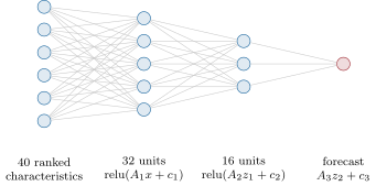
A neural network is a function built by composing parametrised linear maps with fixed nonlinear functions. A multilayer perceptron (MLP) is the fully connected case: $z_0 = x$ , $z_l = \mathrm{act}(A_lz_{l-1} + c_l)$ for $l = 1,\dots,L$ , and $f_\theta(x) = A_{L+1}z_L + c_{L+1}$ , with parameters $\theta = (A_l, c_l)_l$ . The activation function $\mathrm{act}$ is applied coordinate by coordinate; the usual one is $\mathrm{relu}(u) = \max(u, 0)$ .

**Figure 7.1.** The chapter’s small network (drawn with fewer units than it has): 40 inputs, hidden layers of 32 and 16 units, one output, about 1 850 parameters. The larger network adds a first layer of 64 units.

Definition 7.2 (Backpropagation, mini-batch, epoch)

Backpropagation computes the gradient of the loss with respect to every parameter of a network by reverse-mode algorithmic differentiation (Book 4, chapter 28): one forward pass stores the layers’ values, one backward pass propagates $\partial\mathcal L/\partial z_l$ from the output to the input. A mini-batch is the random subset of training rows on which one gradient step is computed; an epoch is one pass over the training set in mini-batches.

The cost of the gradient is a small multiple of the cost of the forward pass, whatever the number of parameters: that is Book 4’s result on reverse mode, and it is why networks can have millions of parameters. The chapter’s networks have two and five thousand and fit in about a second on one CPU thread.

7.2 Optimisers, normalisation and regularisation

Definition 7.3 (Adam, weight decay)

Adam is stochastic gradient descent (Book 4, chapter 24) with a per-parameter step: with gradient $g_k$ at step $k$ , it keeps averages $m_k = \beta_1m_{k-1} + (1-\beta_1)g_k$ and $v_k = \beta_2v_{k-1} + (1-\beta_2)g_k^2$ and moves $\theta$ by $-\eta\,\hat m_k/(\sqrt{\hat v_k} + \epsilon)$ , where hats undo the averages’ bias towards zero (Kingma and Ba). Weight decay shrinks every weight by $\eta\lambda\theta$ at each step, apart from the gradient step (AdamW, Loshchilov and Hutter); for plain gradient descent it is a ridge penalty.

Definition 7.4 (Dropout, batch and layer normalisation)

Dropout sets each hidden unit to zero with probability $d$ during training, scaling the others by $1/(1 - d)$ , and uses the full network at prediction. Batch normalisation standardises each hidden unit over the rows of the mini-batch (running averages at prediction); layer normalisation standardises the units of each row, independently of the batch.

The chapter’s data are chapter 4’s panel (500 stocks, forty ranked characteristics with factor risk, a ceiling of 0.71%): the networks are trained on months 0 to 199 with early stopping on months 201 to 239 (chapter 5’s rule, one month purged), and scored on the ten test years with firm.mlbase’s report, exactly as chapter 4’s models were. Early stopping stops them after two to four epochs (Figure 7.2): on data this noisy, the validation score peaks almost at once, and every later epoch fits more noise than signal.

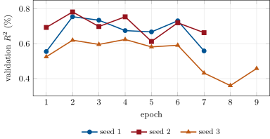
Validation R-squared of the small network after each epoch, three seeds; training stops five epochs after the best. The seeds peak at epochs 2, 2 and 4. Data: ml_nets.fitted. — **Figure 7.2.** Validation R-squared of the small network after each epoch, three seeds; training stops five epochs after the best. The seeds peak at epochs 2, 2 and 4. Data: `ml_nets.fitted`.

With three seeds each, dropout of 0.2 raises the mean test IC from 0.059 to 0.062, weight decay of 0.01 changes nothing at this scale, and both normalisations hurt: batch normalisation to 0.052, layer normalisation to 0.056. Normalising hidden units helps deep networks train; these are shallow, their inputs are already ranks, and a batch’s statistics are one more source of noise. The differences are a few thousandths of IC, comparable to the seed noise measured next, and three seeds per variant is too few to rank them with confidence.

7.3 Seeds as a source of variance

Ten seeds of the small network (32 and 16 units) score test ICs from 0.057 to 0.065, with a mean of 0.0601 and a standard deviation of 0.0023; ten seeds of the larger one (64, 32 and 16) average 0.0619 (Figure 7.3). Their R-squared varies far more than their IC, from 0.08% to 0.30% for the small network: the seed moves the scale of the forecasts, which R-squared punishes and a ranking ignores (chapter 1). The decile portfolio’s net Sharpe ratio goes from 1.37 to 1.78.

Proposition 7.5 (How many seeds a comparison needs)

If two architectures’ scores vary across seeds with standard deviation $s$ , independently, and their means differ by $\delta$ , the difference of their $n$ -seed averages has standard error $s\sqrt{2/n}$ , so it reaches two standard errors when $n \ge 8s^2/\delta^2$ .

Proof. $\Var(\bar a - \bar b) = s^2/n + s^2/n$ ; solve $\delta = 2s\sqrt{2/n}$ for $n$ . ∎

With $s = 0.0024$ (pooled) and $\delta = 0.0019$ , the comparison needs 14 seeds per architecture. A single run of each, the usual practice, compares two draws whose difference has a standard error of 0.0035, almost twice the effect.

Definition 7.6 (Deep ensemble)

A deep ensemble averages the predictions of networks of the same architecture trained from different random seeds on the same data (Lakshminarayanan, Pritzel and Blundell, 2017).

Averaging removes the variance the seeds put in. The ten-seed ensemble of the small network scores an IC of 0.066, above every one of its members, with an R-squared of 0.32% and a net Sharpe ratio of 1.73; the ensemble of the larger network scores 0.066 as well. The architecture question the two researchers argued about disappears once each network is averaged over its seeds: the averaging bought what the architecture could not. It is Proposition 5.3 again, with seeds in the role of bootstrap samples.

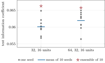
Test IC of ten seeds of two architectures on chapter 4’s panel, their means, and the IC of each ten-seed ensemble. Data: ml_nets.seed_study and ml_nets.ensemble. — **Figure 7.3.** Test IC of ten seeds of two architectures on chapter 4’s panel, their means, and the IC of each ten-seed ensemble. Data: `ml_nets.seed_study` and `ml_nets.ensemble`.

7.4 Ensembles

A seed ensemble costs $n$ trainings and nothing else, and it is embarrassingly parallel. It also gives something a single network cannot: the spread of its members’ forecasts for each row, which chapter 11 uses as a measure of the model’s own uncertainty. Ensembles of different architectures, or of networks with boosted trees and a ridge regression (stacking, Book 7, chapter 14), go further when the members’ errors are less correlated than seeds’ are.

Method 7.7 (Training a network on noisy tabular data)

Rank the inputs by date; scale the target by its training standard deviation.
Start small (two hidden layers, tens of units), with AdamW, a learning rate near $10^{-3}$ , and early stopping on a purged validation block.
Fix every source of randomness (initialisation, dropout, batch order) to one seed per run; train several seeds of anything you compare, and report the mean and the spread.
Deploy the seed ensemble, not the best seed.
Compare with ridge and boosted trees on the same months with the same report.

7.5 Networks against boosting on tabular data

The comparison with chapter 4 is on equal terms: same panel, same test years, same report. A single small network (IC 0.060, net Sharpe ratio 1.37–1.78 across seeds) is ridge regression’s equal (0.060, 1.59); its ten-seed ensemble (0.066, 1.73) matches the lasso’s IC and trails the firm’s default boosted trees (0.075, 2.02). Gu, Kelly and Xiu found networks slightly ahead of trees on real US stocks with sixty years of data, and Grinsztajn, Oyallon and Varoquaux trees ahead of networks on most tabular benchmarks: on panels of ranked characteristics the two families are close, the network needs an ensemble to be competitive, and the tree ensemble is cheaper to tune.

7.6 Tutorial: twenty seeds

Goal. Train small and larger networks with ten seeds each, ensemble them, try four regularisers, and compare with ridge and boosted trees. End state: Figures 7.2 and 7.3, the chapter’s numbers.

The deterministic training loop: one generator for the batch order, the seed for initialisation and dropout, early stopping on the validation loss.

def fit(X, y, Xv, yv, hidden=(32, 16), dropout: float = 0.0, norm=None, lr: float = 1e-3, weight_decay: float = 0.0,
        batch: int = 512, epochs: int = 30, patience: int = 5, seed: int = 1, activation: str = "relu") -> Fitted:
    set_determinism()
    g = torch.Generator().manual_seed(seed)
    torch.manual_seed(seed)
    X = np.asarray(X, np.float32)
    mu, sd = X.mean(axis=0), X.std(axis=0) + 1e-8
    ysd = float(np.std(y)) or 1.0
    Xt = torch.as_tensor((X - mu) / sd)
    yt = torch.as_tensor(np.asarray(y, np.float32) / ysd)
    Xvt = torch.as_tensor((np.asarray(Xv, np.float32) - mu) / sd)
    yvt = torch.as_tensor(np.asarray(yv, np.float32) / ysd)
    model = MLP(X.shape[1], hidden, dropout, norm, activation)
    opt = torch.optim.AdamW(model.parameters(), lr=lr, weight_decay=weight_decay)
    best, best_state, best_ep, bad, hist = np.inf, None, 0, 0, []
    n = len(Xt)
    for ep in range(epochs):
        model.train()
        perm = torch.randperm(n, generator=g)
        for i in range(0, n, batch):
            idx = perm[i:i + batch]
            if len(idx) < 2:
                continue
            opt.zero_grad()
            loss = ((model(Xt[idx]) - yt[idx]) ** 2).mean()
            loss.backward()
            opt.step()
        model.eval()
        with torch.no_grad():
            v = float(((model(Xvt) - yvt) ** 2).mean())
        hist.append(v)
        if v < best - 1e-7:
            best, best_state, best_ep, bad = v, copy.deepcopy(model.state_dict()), ep + 1, 0
        else:
            bad += 1
            if bad >= patience:
                break
    model.load_state_dict(best_state)
    return Fitted(model, mu, sd, ysd, hist, best_ep)

Listing 7.1. A deterministic training loop with early stopping. code/firm/nettab/firm_nettab.py

Run ml_nets.seed_study(), ensemble(), ablation(), baselines() and fig_nets.py.

What to change next. Train with 30 seeds per architecture and check Proposition 7.5’s prediction; replace ReLU by tanh and see whether the seed spread changes.

7.7 Build: the firm’s tabular networks

Purpose. Every network the firm trains on tabular data is reproducible bit for bit and compared across seeds.

Interface. set_determinism(threads), MLP(p, hidden, dropout, norm, activation), fit(X, y, Xv, yv, hidden, dropout, norm, lr, weight_decay, batch, epochs, patience, seed) -> Fitted with predict, history, best_epoch, state_hash(); SeedEnsemble(seeds, **kw).

Rules. One thread, deterministic algorithms, every random draw from the run’s seed; inputs standardised with training statistics stored in the model; the validation block purged by the caller.

Acceptance tests. code/firm/nettab/tests/: two runs with one seed give identical weight hashes, two seeds different ones; the network learns a planted nonlinear function; early stopping keeps the best epoch’s weights; the ensemble averages its members.

Stretch. Mixed-precision training and a data loader for larger panels (chapter 23); export of the weights for chapter 26’s quantised inference.

Sources and further reading

D. P. Kingma and J. Ba, “Adam: a method for stochastic optimization”, ICLR, 2015.
I. Loshchilov and F. Hutter, “Decoupled weight decay regularization”, ICLR, 2019.
N. Srivastava, G. Hinton, A. Krizhevsky, I. Sutskever and R. Salakhutdinov, “Dropout: a simple way to prevent neural networks from overfitting”, JMLR 15, 2014.
S. Ioffe and C. Szegedy, “Batch normalization”, ICML, 2015; J. L. Ba, J. R. Kiros and G. E. Hinton, “Layer normalization”, arXiv, 2016.
B. Lakshminarayanan, A. Pritzel and C. Blundell, “Simple and scalable predictive uncertainty estimation using deep ensembles”, NeurIPS, 2017.
D. E. Rumelhart, G. E. Hinton and R. J. Williams, “Learning representations by back-propagating errors”, Nature 323, 1986.

7.8 Exercises

Exercise 7.1 ★

Count the parameters of an MLP with 40 inputs, hidden layers of 32 and 16 units, and one output. And with a first layer of 64 units added?

Solution

Solution of Exercise 7.1.

$40\times32 + 32 + 32\times16 + 16 + 16 + 1 = 1\,857$ . With a first layer of 64: $40\times64 + 64 + 64\times32 + 32 + 32\times16 + 16 + 17 = 5\,249$ .

Exercise 7.2 ★

Two architectures’ test ICs vary across seeds with a standard deviation of 0.003 and differ by 0.001 on average. How many seeds per architecture does a two-standard-error comparison need?

Solution

Solution of Exercise 7.2.

$n \ge 8\times0.003^2/0.001^2 = 72$ seeds per architecture.

Exercise 7.3 ★

With 160 000 training rows and mini-batches of 512, how many gradient steps is one epoch? And the chapter’s 100 000 rows?

Solution

Solution of Exercise 7.3.

$160\,000/512 = 312.5$ , so 313 steps; the chapter’s $200\times500 = 100\,000$ rows give 196 steps an epoch.

Exercise 7.4 ★★

Why does the seed move R-squared (0.08% to 0.30%) so much more than the IC (0.057 to 0.065)?

Solution

Solution of Exercise 7.4.

The IC depends only on the ranking of the forecasts; R-squared also on their scale. Different seeds stop at different epochs with forecasts spread more or less widely around a similar ranking, and the scale error enters R-squared quadratically (Proposition 1.6).

Exercise 7.5 ★★

Why can batch normalisation hurt a shallow network on ranked inputs, and what would you expect for a deep one?

Solution

Solution of Exercise 7.5.

Batch normalisation standardises each unit with the batch’s own statistics, which are noisy estimates on 512 rows of mostly noise, and it couples the rows of a batch; a shallow network on ranked inputs gains nothing from better conditioning in exchange. In a deep network normalisation keeps the layers’ scales stable and usually makes training possible at all; its noise is then a price worth paying.

Exercise 7.6 ★★

Find the flaw. “We trained twenty seeds and deployed the one with the best validation score.”

Solution

Solution of Exercise 7.6.

The best of twenty validation scores is selected noise (Proposition 3.2): the chosen seed is not better out of sample than the others. Deploy the twenty-seed ensemble, which is.

Exercise 7.7 ★★★

Coding. Compute the IC of ensembles of the first 2, 5 and 10 seeds of the small network. How much of the gain from one to ten seeds do two seeds already buy?

Solution

Solution of Exercise 7.7.

ensemble(n): one seed 0.0602, two 0.0625, five 0.0659, ten 0.0662. Two seeds buy $(0.0625 - 0.0602)/(0.0662 - 0.0602) = 38\%$ of the gain, five seeds 95%.

Exercise 7.8 ★★★

Show that for one ReLU layer and squared loss, backpropagation’s gradient with respect to $A_1$ is $\sum_i (\partial\ell_i/\partial z_{1,i})\odot\mathbf 1\{A_1x_i + c_1 > 0\}\,x_i^\top$ , and count its cost against the forward pass.

Solution

Solution of Exercise 7.8.

With $z_1 = \mathrm{relu}(A_1x + c_1)$ and the forecast linear in $z_1$ , the chain rule gives $\partial\ell_i/\partial A_1 = (\partial\ell_i/\partial z_{1,i}\odot\mathbf 1\{A_1x_i + c_1 > 0\})\,x_i^\top$ , the ReLU’s derivative being the indicator. The backward pass is one matrix-vector product per layer, as the forward pass is, plus elementwise products: a small constant times the forward cost, independent of the number of parameters (Book 4, chapter 28).

7.9 Problem: Twenty Seeds

Problem 7.1

Weekend problem — a network as a random variable

Chapter 4’s panel; networks trained on months 0–199, stopped on months 201–239, scored on months 240–359.

Part I — Training.

How many parameters do the two networks have?
After how many epochs does early stopping stop them, and why so early?
What do dropout, weight decay and the two normalisations do to the IC?
Why are three seeds per variant too few to rank them?

Part II — Seeds.

What range of IC, R-squared and net Sharpe ratio do ten seeds of the small network cover?
What are the two architectures’ mean ICs, the gap, and the pooled seed standard deviation?
How many seeds per architecture does a two-standard-error comparison need?
What is the standard error of a comparison of one run of each?

Part III — Ensembles.

What do the two ten-seed ensembles score?
Why does the ensemble beat every member?
What happens to the architecture question once each network is ensembled?
What does an ensemble give beyond a better forecast?

Part IV — The verdict.

How do the networks compare with ridge, the lasso and boosted trees on the same months?
State the named result: the seed standard deviation of the test IC against the architecture gap, and the number of seeds needed to resolve it at two standard errors.
Which model would you deploy, and in what form?
What should a research log record about a network?
How would the picture change with sixty years of data?
What does the state hash guarantee, and what does it not?
Where does the randomness of a network’s training come from?
In one sentence: what is a network trained once on noisy data?

Solution

Solution of Problem 7.1.

1 857 and 5 249.
After two to four epochs: the validation score peaks almost at once on data this noisy, and later epochs fit noise.
Dropout 0.2 raises the three-seed mean IC from 0.059 to 0.062; weight decay 0.01 changes nothing; batch normalisation lowers it to 0.052, layer normalisation to 0.056.
The seed standard deviation (0.0024) is comparable to the differences, so three seeds give standard errors of the same size as the effects.
IC 0.057 to 0.065, R-squared 0.08% to 0.30%, net Sharpe ratio 1.37 to 1.78.
0.0601 and 0.0619; gap 0.0019; pooled standard deviation 0.0024.
14 per architecture.
$0.00244\sqrt2 = 0.0035$ , almost twice the effect.
0.066 each (the small ensemble: R-squared 0.32%, net Sharpe ratio 1.73).
Averaging removes the seed-specific part of each member’s error (Proposition 5.3).
It disappears: both ensembles score 0.066.
The spread of the members’ forecasts for each row, a measure of the model’s own uncertainty (chapter 11).
A single network equals ridge (IC 0.060); the ensemble equals the lasso’s IC (0.066) and trails the default boosted trees (0.075, net Sharpe ratio 2.02).
Named result: the seed standard deviation of the test IC, 0.0024, exceeds the architecture gap, 0.0019; resolving it at two standard errors needs 14 seeds per architecture, and a ten-seed ensemble (0.066) beats both architectures’ single runs.
The boosted trees; if a network, its seed ensemble, never its best seed.
Architecture, every hyperparameter, the seeds, the validation block, the best epoch of each seed, the state hashes, and the spread of the results.
More data lower the variance of each fit, so seeds matter less and larger networks can pay for themselves.
That the same code, data and seed produce the same weights; not that the result is good, nor that another seed would agree.
The initial weights, the dropout masks and the order of the mini-batches (and, on accelerators, non-deterministic kernels).
One draw from a distribution of models, whose spread must be measured before its mean is compared.

7.10 Interview questions

Interview question 7.1 ★ mle

What does backpropagation compute, and why is it cheap?

Solution

Solution of Interview question 7.1.

The gradient of the loss with respect to every weight, by the chain rule applied from the output backwards (reverse-mode differentiation). Its cost is a small multiple of one forward pass, because each layer’s derivative is reused by all the layers before it.

What the interviewer is looking for: reverse mode and the cost argument.

Interview question 7.2 ★ mle, researcher

Explain the difference between Adam and AdamW.

Solution

Solution of Interview question 7.2.

Adam with an $\ell_2$ penalty adds $\lambda\theta$ to the gradient, which is then rescaled by Adam’s per-parameter step, so weights with large gradient variance are barely penalised; AdamW shrinks the weights directly, outside the adaptive step, which restores weight decay’s meaning.

What the interviewer is looking for: the interaction between the penalty and the adaptive scaling.

Interview question 7.3 ★★ researcher, mle

Your new architecture beats the old one by 0.003 of IC in one run each. What do you do before believing it?

Solution

Solution of Interview question 7.3.

Train several seeds of each (Proposition 7.5 says how many), compare means with the standard error of the difference, and compare the seed ensembles; check the gain on another period.

What the interviewer is looking for: seeds as noise and a proper two-sample comparison.

Interview question 7.4 ★★ mle

How do you make a PyTorch training run reproducible on CPU? What can still break reproducibility?

Solution

Solution of Interview question 7.4.

Seed every generator (torch, NumPy, the batch sampler), use one thread and deterministic algorithms (torch.use_deterministic_algorithms), fix library versions, and hash the weights. Different library versions, hardware, thread counts or BLAS back ends can still change results in the last bits.

What the interviewer is looking for: every source of randomness and of floating-point non-associativity.

Interview question 7.5 ★★ researcher

Neural network or gradient boosting for a cross-sectional return model? Argue both sides.

Solution

Solution of Interview question 7.5.

Trees: strong defaults, cheap tuning, robust to scaling, monotonic constraints, fast inference, usually at least as good on ranked characteristics. Networks: smooth interactions, embeddings, joint training with other objectives, benefits from very large data, and ensembles that estimate their own uncertainty. On a monthly panel, start with trees and add a network ensemble if it improves the stack.

What the interviewer is looking for: a balanced argument tied to data size and use.

Interview question 7.6 ★★★ researcher, mle

Why does averaging networks trained from different seeds improve the forecast, and when does it stop helping?

Solution

Solution of Interview question 7.6.

Each network’s error has a part common to all seeds (what the data and architecture allow) and a seed-specific part; averaging removes the second, by $\rho\sigma^2 + (1-\rho)\sigma^2/B$ . It stops helping when the seed-specific part is gone, after a handful of seeds here: the members’ remaining error is correlated.

What the interviewer is looking for: the variance decomposition and its floor.

Terms defined in this chapter

See all 2333 terms in the glossary