Machine Learning for Markets · Machine learning

22From Prediction to Portfolio

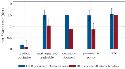
The forecast with the lowest error of the chapter’s experiment produces a portfolio with a net Sharpe ratio of 0.19; a forecast with a slightly higher error produces one of 1.52. The first was fitted on every name and learned the strong signal in the names the desk cannot trade; the second was fitted on the names it can, where the signal is weaker and different. A forecast is an input to a decision, and the loss it is trained on should care about what the decision does with it. This chapter compares the three ways to make it care: train the forecast only where the portfolio uses it, train it through the portfolio rule (decision-focused learning), or skip the forecast and learn the portfolio rule directly (parametric portfolio policies). It ends with the price of the second and third: they fit noise that least squares would ignore.

22.1 Why the forecast loss is not the trading loss

Definition 22.1 (Predict-then-optimise)

Predict-then-optimise fits a forecast by a statistical loss (mean squared error, a likelihood) and passes it to an optimiser that chooses the portfolio; the two steps are fitted separately.

Book 7 (chapter 15) measured the loss between forecast and portfolio through the transfer coefficient; the loss here is earlier, in the forecast itself. Mean squared error weighs every name and every period equally; the portfolio’s profit depends on the forecast only where the optimiser trades, in proportion to the positions it takes, and after costs. When the forecast model is correctly specified, least squares estimates the true relation and the difference does not matter. When it is not, the model spends its limited flexibility on the errors that matter most to the loss, which need not be those that matter to the portfolio (Elmachtoub and Grigas, 2022).

The chapter’s panel makes that concrete. Two hundred names carry four characteristics that follow slow AR(1) processes. In the hundred names the desk cannot trade (too small, restricted), the first characteristic predicts next period’s return strongly (0.3% per unit); in the hundred it can, only the second does, weakly (0.08%). Returns have 3% of noise per period. The forecast is linear in the characteristics with one coefficient each for all names, so it cannot be right everywhere. The portfolio rule is mean-variance on the tradeable names with a quadratic cost proxy,

w_{i,t} = \frac{\hat\mu_{i,t} + 2\kappa w_{i,t-1}}{\gamma\sigma^2 + 2\kappa},

with $\gamma = 20$ , $\sigma = 3\%$ and $\kappa$ equal to the linear cost of 5 basis points that net returns pay on every change in weight. Five pairs of independent panels, 1 500 periods each, give training and test data.

Least squares on all names puts a coefficient of 1.51 (in units of 0.1%) on the first characteristic and 0.43 on the second (Figure 22.2): it has learned mostly the untradeable signal. Out of sample its mean squared error is lower than that of least squares on the tradeable names alone (9.007 against 9.031, in units of $10^{-4}$ ), and higher on the names the desk trades (8.987 against 8.962): the better forecast by the usual measure is the worse one where it is used.

22.2 Losses aligned with profit and loss

The simplest alignment is to fit the forecast on the data the decision uses: least squares on the tradeable names finds the second characteristic (0.83 against a true 0.80) and ignores the first. More generally, a weighted loss can weigh each name by the size of the position the optimiser would take, or by its liquidity, and a loss on the portfolio’s return rather than on the forecast aligns the two completely.

Definition 22.2 (Decision-focused learning, differentiable optimisation layer)

Decision-focused learning trains a forecast by the quality of the decisions made with it: the forecast is passed through the optimiser and the loss is computed on the decision’s outcome (Donti, Amos and Kolter, 2017). It needs a differentiable optimisation layer: an optimiser whose solution can be differentiated with respect to its inputs, in closed form as here, by implicit differentiation of the optimality conditions of a quadratic programme (Amos and Kolter, 2017), or for general convex problems (Agrawal and co-authors, 2019).

22.3 Parametric portfolio policies

Definition 22.3 (Parametric portfolio policy)

A parametric portfolio policy writes the weights directly as a function of the names’ characteristics, $w_{i,t} = \theta^\top x_{i,t}/N$ around a benchmark, and chooses $\theta$ to maximise the investor’s average utility over the sample (Brandt, Santa-Clara and Valkanov, 2009); there is no forecast, and the characteristics’ covariances with returns enter only through the portfolio’s outcome.

The chapter trains both by gradient ascent on the Sharpe ratio of net returns over windows of 100 periods (Listing 22.2), starting from the all-names least-squares coefficients: the decision-focused forecast through the mean-variance rule, the parametric policy without its smoothing. Table 22.1 and Figure 22.1 give the test results.

coefficients chosen by	net Sharpe	(s.d., 5 pairs)	gross Sharpe	turnover
least squares, all names (predict, then optimise)	0.19	0.09	0.60	2.95
least squares, tradeable names	1.52	0.23	1.92	1.59
decision-focused learning	1.51	0.22	1.92	2.75
parametric portfolio policy	1.49	0.23	1.92	2.90
true coefficients	1.57	0.24	1.97	1.50

Table 22.1. Annualised Sharpe ratios on test panels (52 periods a year) and mean turnover per period (sum of absolute weight changes), means over five train-test pairs. Data: ml_e2e.results.

22.4 Learning through the optimiser

Learning through the decision recovers what predict-then-optimise loses: 1.51 against 0.19, a gap of 1.33 with a standard deviation of 0.18 over the five pairs. It learns the right direction, 1.43 on the second characteristic and almost nothing on the first; the scale is larger than the truth’s because a Sharpe ratio does not depend on it, and the turnover is higher for the same reason. But it does no better than least squares on the tradeable names, which is simpler, faster and turns over less. The gain came from aligning the data with the decision, not from differentiating through the optimiser; here the optimiser is simple enough that the two coincide. Decision-focused learning earns its complexity when the decision’s sensitivity to the forecast varies in ways a weight cannot express: constraints that bind for some names and not others, costs that depend on the trade, risk that couples the names.

Net Sharpe ratio on test panels by the way the forecast’s coefficients were chosen, mean and standard deviation over five train-test pairs, with ample data and with little data and many useless characteristics. Data: ml_e2e.summary. — **Figure 22.1.** Net Sharpe ratio on test panels by the way the forecast’s coefficients were chosen, mean and standard deviation over five train-test pairs, with ample data and with little data and many useless characteristics. Data: `ml_e2e.summary`.

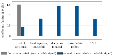
The forecast’s coefficients on the two informative characteristics, means over five training panels. Data: ml_e2e.results. — **Figure 22.2.** The forecast’s coefficients on the two informative characteristics, means over five training panels. Data: `ml_e2e.results`.

22.5 When end-to-end learning overfits

A loss computed on the portfolio’s net Sharpe ratio is a noisy, low-dimensional summary of the data; fitting many parameters to it is fitting to noise. With 300 training periods and sixteen useless characteristics added, least squares on the tradeable names still reaches 1.04 out of sample, decision-focused learning 0.89 and the parametric policy 0.87 (Figure 22.1), with higher turnover (3.49 against 1.88): the end-to-end fits spent their freedom on characteristics that happened to pay in the training sample. Even with 1 500 periods, the decision-focused coefficients on the two useless characteristics of the first panel were $-0.44$ and 0.20, against $-0.22$ and 0.13 for least squares on the tradeable names. The remedies are those of any small-sample fit: fewer parameters, penalties, early stopping on a validation block, and a least-squares starting point that the end-to-end fit must beat on held-out data.

Method 22.4 (From forecast to portfolio)

Fit forecasts on the names, periods and horizons the portfolio uses, weighted by how much the portfolio depends on them.
Evaluate forecasts by the net performance of the portfolio built from them, never by forecast error alone.
Use decision-focused learning or parametric policies when the decision’s sensitivity to the forecast cannot be expressed as a weight, with strong regularisation and a least-squares benchmark.
Report the spread across independent samples; a gap smaller than it is no gap.

22.6 Tutorial: the loss that pays

Goal. Compare predict-then-optimise, aligned least squares, decision-focused learning and a parametric policy on five train-test pairs, then with little data and many characteristics. End state: Table 22.1, Figures 22.1 and 22.2.

The portfolio rule and its evaluation.

def mv_layer(mu, w_prev, kappa, gamma=GAMMA, sigma=SIGMA):
    """argmax_w mu w - gamma/2 sigma^2 w^2 - kappa (w - w_prev)^2, name by name."""
    return (mu + 2 * kappa * w_prev) / (gamma * sigma**2 + 2 * kappa)


def _weights(policy, mu, w, cost, gamma, sigma):
    if policy == "mv":
        return mv_layer(mu, w, cost, gamma, sigma)
    return mu / (gamma * sigma**2)                                       # parametric policy: no smoothing


def run(b, X, R, tradeable, cost=COST, gamma=GAMMA, sigma=SIGMA, policy="mv"):
    """Trade the tradeable names period by period; net returns pay cost times the absolute change in weights."""
    T, N, _ = X.shape
    w = np.zeros(N)
    net, gross, turn = np.empty(T), np.empty(T), np.empty(T)
    for t in range(T):
        wn = np.where(tradeable, _weights(policy, X[t] @ b, w, cost, gamma, sigma), 0.0)
        gross[t] = wn @ R[t]
        turn[t] = np.abs(wn - w).sum()
        net[t] = gross[t] - cost * turn[t]
        w = wn
    sr = lambda x: float(x.mean() / x.std() * math.sqrt(52))            # noqa: E731
    return {"net": sr(net), "gross": sr(gross), "turnover": float(turn.mean())}

Listing 22.1. A differentiable mean-variance rule with a cost proxy, and the net-return evaluation. code/firm/e2eport/firm_e2eport.py

Learning through the decision.

def train_decision(X, R, tradeable, init, policy="mv", epochs=20, lr=0.02, window=100, seed=0, cost=COST,
                   gamma=GAMMA, sigma=SIGMA):
    """Maximise the Sharpe ratio of net returns over windows of `window` periods by gradient ascent through the
    portfolio rule; coefficients in units of 0.1%."""
    torch.set_num_threads(1)
    torch.use_deterministic_algorithms(True)
    torch.manual_seed(seed)
    Xt = torch.as_tensor(X[:, tradeable], dtype=torch.float32)
    Rt = torch.as_tensor(R[:, tradeable], dtype=torch.float32)
    th = torch.tensor(np.asarray(init) * 1e3, dtype=torch.float32, requires_grad=True)
    opt = torch.optim.Adam([th], lr=lr)
    for _ in range(epochs):
        for s in range(0, len(Xt) - window + 1, window):
            w = torch.zeros(Xt.shape[1])
            nets = []
            for t in range(s, s + window):
                wn = _weights(policy, Xt[t] @ (1e-3 * th), w, cost, gamma, sigma)
                nets.append(wn @ Rt[t] - cost * torch.abs(wn - w).sum())
                w = wn
            n = torch.stack(nets)
            loss = -n.mean() / n.std()
            opt.zero_grad()
            loss.backward()
            opt.step()
    return 1e-3 * th.detach().numpy()

Listing 22.2. Gradient ascent on the net Sharpe ratio through the rule. code/firm/e2eport/firm_e2eport.py

Run ml_e2e.results(), overfit(), summary(), forecast_errors() and fig_e2e.py (about 45 seconds on one core).

What to change next. Add a name-level position limit that binds for some names and see whether aligned least squares can still match decision-focused learning; add early stopping on a validation block to the end-to-end fit.

22.7 Build: end-to-end portfolios

Purpose. Forecasts judged and, where it pays, trained by the portfolios they produce.

Interface. char_panel(seed, T, N, K, n_noise, phi), mv_layer(mu, w_prev, kappa, gamma, sigma), run(b, X, R, tradeable, cost, gamma, sigma, policy), least_squares(X, R, rows), train_decision(X, R, tradeable, init, policy, epochs, lr, window, seed).

Rules. Every end-to-end result is reported against aligned least squares on the same held-out data, with its spread over independent samples.

Acceptance tests. code/firm/e2eport/tests/: the closed-form layer equals Book 7’s firm.portcons solution when costs are zero; the layer’s gradient matches finite differences; the evaluation charges costs on weight changes; decision-focused training on a clean problem recovers the direction of the true coefficients.

Stretch. A general quadratic-programme layer by implicit differentiation, with a factor risk model; name-level limits; early stopping.

Sources and further reading

M. W. Brandt, P. Santa-Clara and R. Valkanov, “Parametric portfolio policies: exploiting characteristics in the cross-section of equity returns”, Review of Financial Studies 22(9), 2009.
A. N. Elmachtoub and P. Grigas, “Smart ‘predict, then optimize”’, Management Science 68(1), 2022.
P. L. Donti, B. Amos and J. Z. Kolter, “Task-based end-to-end model learning in stochastic optimization”, arXiv:1703.04529, 2017.
B. Amos and J. Z. Kolter, “OptNet: differentiable optimization as a layer in neural networks”, arXiv:1703.00443, 2017.
A. Agrawal and co-authors, “Differentiable convex optimization layers”, arXiv:1910.12430, 2019.
A. Butler and R. H. Kwon, “Integrating prediction in mean-variance portfolio optimization”, Quantitative Finance 23(3), 2023.

22.8 Exercises

Exercise 22.1 ★

Derive the rule $w = (\mu + 2\kappa w_{\mathrm{prev}})/(\gamma\sigma^2 + 2\kappa)$ from the one-name objective. What does it become with $\kappa = 0$ and as $\kappa\to\infty$ ?

Solution

Solution of Exercise 22.1.

Maximise $\mu w - \frac\gamma2\sigma^2w^2 - \kappa(w - w_{\mathrm{prev}})^2$ : the first-order condition $\mu - \gamma\sigma^2w - 2\kappa(w - w_{\mathrm{prev}}) = 0$ gives the rule. With $\kappa = 0$ it is the mean-variance weight $\mu/(\gamma\sigma^2)$ ; as $\kappa\to\infty$ the weight stays at $w_{\mathrm{prev}}$ .

Exercise 22.2 ★

With the chapter’s parameters, what fraction of the gap to its target does a name’s weight close each period?

Solution

Solution of Exercise 22.2.

The rule is $w = a\,\mu/(\gamma\sigma^2) + (1 - a)w_{\mathrm{prev}}$ with $a = \gamma\sigma^2/(\gamma\sigma^2 + 2\kappa) = 0.018/(0.018 + 0.001) = 0.947$ : 95% of the gap is closed each period; the cost proxy slows the portfolio only a little.

Exercise 22.3 ★

Why does a Sharpe-ratio loss leave the scale of the coefficients undetermined, and what does that do to turnover?

Solution

Solution of Exercise 22.3.

Multiplying every return by a constant leaves the Sharpe ratio unchanged, so any scale of the coefficients with the same direction is equally good up to the effect of costs; gradient ascent drifts in scale, larger positions trade more, and the decision-focused turnover (2.75) exceeds aligned least squares’ (1.59) at the same Sharpe ratio.

Exercise 22.4 ★★

Explain why the all-names least-squares forecast has the lower error overall and the higher error on the tradeable names.

Solution

Solution of Exercise 22.4.

Squared error is dominated by the untradeable names, where the first characteristic’s signal is strong; fitting it lowers the error there more than it raises it among the tradeable names, where that coefficient is pure error. Least squares on the tradeable names fits only where it is scored by the portfolio.

Exercise 22.5 ★★

When would decision-focused learning beat least squares on the tradeable names in this setting?

Solution

Solution of Exercise 22.5.

When the portfolio’s sensitivity to the forecast differs across tradeable names or periods in a way a weight cannot express: binding position limits for some names, costs that depend on trade size, a factor risk model that nets positions, a forecast that feeds a non-linear rule. Then the errors that matter are not simply the errors on the traded names.

Exercise 22.6 ★★

Find the flaw. “We trained the network end to end on the portfolio’s Sharpe ratio and got 3.1 in the backtest, against 1.2 for the forecast trained on returns, so end-to-end training is worth it.”

Solution

Solution of Exercise 22.6.

The comparison is in the backtest the end-to-end model was fitted on, or selected on: a loss on the portfolio’s Sharpe ratio is a strong incentive to fit noise. Compare on held-out data, against a forecast trained on the traded names, with the spread over independent samples; the chapter’s small-sample case shows the end-to-end fit losing out of sample.

Exercise 22.7 ★★★

Coding. Add a ridge penalty to the decision-focused training in the small-sample scenario and choose its strength on a validation block. Does it close the gap to aligned least squares?

Solution

Solution of Exercise 22.7.

Started from least squares on the tradeable names, with the number of epochs chosen on the last 60 training periods, the validation block chooses no end-to-end training at all in three of the five samples; the mean test net Sharpe ratio is 1.04, the same as aligned least squares. Early stopping closes the gap by, mostly, stopping at the start.

Exercise 22.8 ★★★

For the unconstrained mean-variance problem $\max_w\mu^\top w - \frac\gamma2w^\top\Sigma w$ , compute $\partial w^*/\partial\mu$ and explain how the gradient of a portfolio loss flows back to the forecast.

Solution

Solution of Exercise 22.8.

$w^* = \Sigma^{-1}\mu/\gamma$ , so $\partial w^*/\partial\mu = \Sigma^{-1}/\gamma$ . For a loss $L(w^*)$ , $\partial L/\partial\mu = (\partial w^*/\partial\mu)^\top\nabla_wL = \Sigma^{-1}\nabla_wL/\gamma$ , and back-propagation carries it to the forecast’s parameters. The forecast’s error matters in the directions the optimiser amplifies: those of low risk.

22.9 Problem: The Loss That Pays

Problem 22.1

Weekend problem — train on what you trade

The chapter’s panel, portfolio rule and five ways to choose the forecast.

Part I — The setup.

What does each half of the universe contain, and what can the linear forecast represent?
What does the portfolio rule do, and how are costs charged?
What coefficients does least squares on all names learn, and why?
How do the two least-squares forecasts compare by mean squared error?

Part II — The comparison.

Give the net and gross Sharpe ratios and the turnover of the five methods.
What is the gap between decision-focused learning and predict-then-optimise, and its spread?
Why do aligned least squares and decision-focused learning tie?
Why is the parametric policy’s turnover highest?

Part III — Overfitting.

What happens with 300 periods and twenty characteristics?
Which coefficients show the overfit?
What regularisation would you use?
How would you pick between the methods on real data?

Part IV — The verdict.

State the named result: the net Sharpe ratio of predict-then-optimise against decision-focused learning and the parametric policy, with the gap’s spread over seeds.
When is predict-then-optimise enough?
What would make decision-focused learning worth its cost?
How does this relate to the transfer coefficient?
What should a research report on a new forecast contain, after this chapter?
Where do costs enter the training loss, and where should they?
How would you do this with a neural forecast?
In one sentence: what should a forecast be trained to do?

Solution

Solution of Problem 22.1.

Part I.

Untradeable names where the first characteristic predicts strongly, tradeable names where the second predicts weakly; a single linear forecast cannot be right in both.
Mean-variance weights with a quadratic cost proxy on the tradeable names; net returns pay 5 basis points on every change in weight.
1.51 on the first characteristic and 0.43 on the second (0.1% units): mostly the untradeable signal, which dominates the squared error.
All names: 9.007 overall and 8.987 on the tradeable names; tradeable-names fit: 9.031 and 8.962 ( $10^{-4}$ units).

Part II.

Net, gross, turnover: 0.19, 0.60, 2.95; 1.52, 1.92, 1.59; 1.51, 1.92, 2.75; 1.49, 1.92, 2.90; truth 1.57, 1.97, 1.50.
1.33 with a standard deviation of 0.18 over five pairs.
Both learn the second characteristic’s direction; here the only thing the decision adds is which names matter, and a restricted fit says the same.
It has no smoothing: weights move with the characteristics every period.

Part III.

Aligned least squares 1.04, decision-focused 0.89, parametric 0.87, predict-then-optimise 0.09, truth 1.51.
The coefficients on useless characteristics, and turnover of 3.49 against 1.88.
Few parameters, a least-squares start, early stopping on a validation block, penalties on the direction, not only the scale.
On held-out periods and independent samples, by net performance and its spread, with aligned least squares as the benchmark.

Part IV.

The loss that pays. Predict-then-optimise earns a net Sharpe ratio of 0.19, decision-focused learning 1.51 and the parametric policy 1.49; the gap of 1.33 has a standard deviation of 0.18 over five train-test pairs, and least squares on the traded names alone matches the end-to-end methods (1.52).
When the forecast model is well specified, or when it is fitted on the names and periods the decision uses.
Decisions whose sensitivity to the forecast varies in ways a sample restriction or weight cannot capture, and enough data to fit through them.
The transfer coefficient measures what constraints lose between forecast and portfolio; this chapter’s loss happens before, when the forecast learns the wrong thing.
Its net portfolio performance under the desk’s construction and costs, on held-out data, against the incumbent, with turnover and spread.
In the portfolio’s evaluation always; in training through a cost-aware rule or a cost-weighted loss.
The same, with the network in place of the linear forecast, and more regularisation.
To make the portfolio built from it good, net of costs, out of sample.

22.10 Interview questions

Interview question 22.1 ★ researcher

Why can a more accurate forecast produce a worse portfolio?

Solution

Solution of Interview question 22.1.

Accuracy is measured everywhere; profit depends on the forecast only where and as much as the optimiser trades on it, after costs and constraints. A misspecified model trades errors between names, and the loss decides which.

What the interviewer is looking for: misspecification and the mismatch between the loss and the decision.

Interview question 22.2 ★★ researcher, mle

What is decision-focused learning, and how do you differentiate through an optimiser?

Solution

Solution of Interview question 22.2.

Train the forecast by the loss of the decision made with it; differentiate the optimiser’s solution in closed form, by unrolling an iterative solver, or by implicit differentiation of its optimality conditions.

What the interviewer is looking for: the loss and at least one differentiation method.

Interview question 22.3 ★★ researcher

Describe Brandt, Santa-Clara and Valkanov’s parametric portfolio policies. What are their advantages and risks?

Solution

Solution of Interview question 22.3.

Weights are a linear function of characteristics around a benchmark, with coefficients chosen to maximise average utility in sample. Few parameters, no covariance matrix, costs and constraints can enter the utility; but in-sample utility maximisation overfits and the policy form is restrictive.

What the interviewer is looking for: the form, the fitting criterion, and the overfitting risk.

Interview question 22.4 ★★ researcher, trader

How would you include transaction costs in the training of an alpha model?

Solution

Solution of Interview question 22.4.

Evaluate the model by net portfolio returns; fit it on tradeable names, weighted by liquidity or expected position; or train through a cost-aware portfolio rule; and penalise turnover in the forecast (smoothness) where costs are high.

What the interviewer is looking for: net evaluation and at least one way to bring costs into training.

Interview question 22.5 ★★ mle

An end-to-end portfolio network backtests far better than predict-then-optimise. What do you check?

Solution

Solution of Interview question 22.5.

Whether it was evaluated on data used in fitting or selection, its turnover and costs, the spread over seeds and samples, the benchmark (a forecast fitted on the traded names), and the number of parameters against the data.

What the interviewer is looking for: held-out evaluation, a fair benchmark and a spread.

Interview question 22.6 ★★★ researcher

Show how the KKT conditions of a quadratic programme give the derivative of its solution with respect to the linear term.

Solution

Solution of Interview question 22.6.

For $\min\frac12w^\top Qw - \mu^\top w$ subject to $Aw = b$ , the KKT system $Qw - \mu + A^\top\lambda = 0$ , $Aw = b$ is linear; differentiating gives $\begin{pmatrix}Q & A^\top\\ A & 0\end{pmatrix}\begin{pmatrix}dw\\ d\lambda\end{pmatrix} = \begin{pmatrix}d\mu\\ 0\end{pmatrix}$ , so $dw/d\mu$ is the top-left block of the inverse; inequality constraints add the active ones to $A$ (OptNet).

What the interviewer is looking for: the linearised KKT system and active constraints.

Terms defined in this chapter

See all 2333 terms in the glossary