19Deep Hedging and Machine Learning in Pricing

A one-month at-the-money call on a stock whose volatility follows Heston’s model is worth 2.25 on a spot of 100, and one point of implied volatility is worth 0.115 of it. Hedged every day to its Black–Scholes delta with a transaction cost of 5 basis points, the hedge pays 0.123 in costs on average: more than a volatility point, for a trader whose edge is often less. A network that learns when not to trade pays 0.099 and carries less risk. This chapter uses machine learning where derivatives desks use it: to hedge under frictions that the textbook ignores (deep hedging), to replace a slow pricer by a fast approximation (surrogates, and the differential learning that makes them accurate with few samples), and to calibrate a model in one pass. Each is measured against the exact answer that Book 5’s engines provide, and each has a place where it breaks.

19.1 Hedging under frictions as a learning problem

Book 5 (chapter 4) measured the discrete hedging error of the Black–Scholes delta and (chapter 26) the hedging band that transaction costs call for. With costs, the best hedge depends on the current holding (trading back to delta is not worth it if delta has moved little), on the risk the trader is willing to carry, and on everything the model leaves out; there is no closed form beyond asymptotic ones. The problem is a stochastic control problem (Book 4, chapter 9) whose objective is a risk measure of the hedged P&L.

Definition 19.1 (Convex risk measure, entropic risk measure, indifference price)

A convex risk measure $\rho$ assigns to a random P&L $X$ the amount of cash that makes it acceptable, and is monotone, cash-invariant ($\rho(X + c) = \rho(X) - c$) and convex (Föllmer and Schied, 2002); expected shortfall (Book 6, chapter 21) is one. The entropic risk measure is $\rho(X) = \lambda^{-1}\log\E[e^{-\lambda X}]$, the certainty equivalent of exponential utility with risk aversion $\lambda$. The indifference price of a claim is the premium that leaves the seller exactly as well off, by the risk measure, as not selling, each with its best trading strategy: $p = \inf_\delta\rho(-Z + G_\delta) - \inf_\delta\rho(G_\delta)$, where $G_\delta$ is the gain of trading strategy $\delta$ after costs. When the underlying’s price is a martingale, as in the chapter’s simulation, not trading is best without the claim and the second term is zero.

19.2 Deep hedging

Definition 19.2 (Deep hedging)

Deep hedging represents the hedging strategy by a neural network that maps what is observable at each date (time, prices, current holdings) to the new holdings, and trains it on simulated paths to minimise a convex risk measure of the hedged P&L after all frictions (Buehler, Gonon, Teichmann and Wood, 2019).

The chapter’s network (Listing 19.1) is the no-transaction band network of Imaki and co-authors (2021): from the time to maturity and the log-moneyness it outputs a band, and the new holding is the old one clipped into it, so that not trading is the default and the band’s width can be read off. The P&L of selling the call and hedging daily with the underlying is computed on a batch of paths (Listing 19.2), the entropic risk with $\lambda = 1$ is the loss, and 1 000 Adam steps on batches of 2 048 of 20 000 training paths take about fifteen seconds on one core. Every policy is then scored on 20 000 other paths.

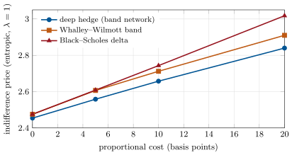
Figure 19.1 is the first half of the chapter’s named result. Without costs the deep hedge’s indifference price is 2.454 against 2.475 for the Black–Scholes delta: under Heston, spot and volatility move together ($\rho = -0.7$) and the network learns a hedge ratio that uses it. With costs of 5, 10 and 20 basis points it rises to 2.558, 2.658 and 2.840; the Black–Scholes delta hedge’s to 2.608, 2.743 and 3.018, and the Whalley–Wilmott band’s (Whalley and Wilmott, 1997) to 2.606, 2.712 and 2.910. Table 19.1 shows the other statistics at 10 basis points. Trained on expected shortfall instead, the network lowers the expected shortfall (3.763 against 3.817) and raises the entropic risk (2.671 against 2.658): the risk measure is part of the model, and each network is best by its own.

policy	entropic risk	expected shortfall 95%	mean cost	standard deviation
deep hedge, entropic	2.658	3.817	2.442	0.643
deep hedge, expected shortfall	2.671	3.763	2.457	0.657
Whalley–Wilmott band	2.712	4.044	2.424	0.703
Black–Scholes delta	2.743	4.090	2.507	0.595
no hedge	8.767	9.992	2.235	2.945

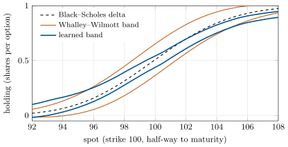
The second half of the named result is the band itself (Figure 19.2). At the money half-way to maturity, the learned band is 0.031 wide in delta at 5 basis points and 0.104 at 20; the Whalley–Wilmott band, $\pm(3cS\Gamma^2/2\lambda)^{1/3}$, is 0.181 and 0.288. The asymptotic formula assumes a trader who watches continuously and trades at the band’s edge; with one decision a day, the position drifts between decisions and a wide band compounds the drift, so the network keeps a narrower band at the money and above it, and a wider one below the money, where the option is nearly worthless to hedge. The formula gives the right idea and the wrong size for this trader; the network finds the size for the trader’s actual schedule and risk measure.

19.3 Surrogate pricers and differential learning

Definition 19.3 (Surrogate model, differential machine learning)

A surrogate model is a fast approximation of a slow function, here a pricer, fitted to its outputs on sampled inputs. Differential machine learning trains the surrogate on the derivatives of the labels with respect to the inputs as well as on the labels, the network’s own derivatives being computed by automatic differentiation (Book 4, chapter 28); with Monte Carlo labels the derivative labels are pathwise (Huge and Savine, 2020).

A risk system that prices a book under thousands of scenarios cannot afford a Fourier integral or a Monte Carlo run per price. The chapter’s surrogate learns the Heston price of a three-month call as a function of the spot (70 to 130) and the initial variance (0.01 to 0.09) from the cheapest labels there are: one simulated path per sample, whose payoff is an unbiased but very noisy price. The differential label is the pathwise derivative of the payoff with respect to the spot, $\mathbf1\{S_T > K\}S_T/S_0$, free once the path exists. Table 19.2 scores both trainings against the Fourier price on 400 test points (Listing 19.3 is the training loop).

	price RMSE		delta RMSE
training samples	standard	differential	standard	differential
256	0.927	0.679	0.066	0.057
1 024	0.436	0.218	0.059	0.021
4 096	0.297	0.279	0.042	0.020

With 1 024 samples the derivative labels halve the price error and cut the delta error by nearly two-thirds; with 4 096 the prices are as good either way but only the differential network’s deltas are. A surrogate’s delta is what the hedger uses, and a network fitted to prices alone has no reason to get its slope right.

19.4 Calibration networks

Definition 19.4 (Deep calibration)

Deep calibration replaces the numerical optimisation of a model’s parameters against market quotes (Book 4, chapter 24) by a network trained on model-generated data: either the inverse map from quotes to parameters (Hernandez, 2016) or a fast forward map from parameters to quotes inside a standard optimiser (Horvath, Muguruza and Tomas, 2021).

The chapter’s network learns the inverse map from fifteen normalised call prices (five strikes, three maturities) to the five Heston parameters, on 4 000 parameter sets drawn uniformly in a box. On 200 test sets, its errors as a share of each parameter’s range are 1.7% for the initial variance, 18.7% for the mean-reversion speed, 9.7% for the long-run variance, 9.0% for the volatility of variance and 9.8% for the correlation; the surfaces re-priced with its answers miss the true ones by 13.2 basis points of spot on average. Speed and long-run variance are poorly identified by three maturities, and the network is as uncertain about them as the data are. On five test surfaces its answer misses the implied volatilities by 0.46 points on average, and Book 5’s Levenberg–Marquardt calibrator, started from it or from a fixed guess, fits them exactly. The network is a fast first guess and a sanity check, not a replacement, on clean data from the model it was trained on; on market data, which no model fits exactly, it has never seen the residuals it will meet.

19.5 Where learned pricing breaks

Three failures recur. Extrapolation: a surrogate or a calibration network outside its training box returns confident numbers with no warning, exactly where a stressed market takes the book; train on boxes wider than any scenario and check inputs against them. Arbitrage: a surrogate’s prices need not be monotone or convex in the strike, and its Greeks can change sign where they should not; constrain the architecture or check the outputs. Model risk: a deep hedge is optimal for the simulator it was trained on, like chapter 17’s agent; train it on several models or randomised parameters, and compare it with the asymptotic band on paths it was not trained on.

Method 19.5 (Machine learning on a derivatives desk)

1. Keep the exact pricer as the reference; every surrogate is validated against it on a grid wider than the book’s scenarios, prices and Greeks both.
2. Train surrogates with differential labels when derivatives are cheap (pathwise or by automatic differentiation).
3. Use calibration networks as starting points and checks; the optimiser has the last word.
4. Train deep hedges on the desk’s own frictions and risk measure, and compare with the closed-form band out of sample and across models.

19.6 Tutorial: hedging with frictions

19.7 Build: deep hedging and learned pricers

19.8 Exercises

Exercise 19.1 ★

Show that the entropic risk measure is cash-invariant: $\rho(X + c) = \rho(X) - c$. What is $\rho$ of a constant?

Solution

Solution of Exercise 19.1.

$\rho(X + c) = \lambda^{-1}\log\E[e^{-\lambda X}e^{-\lambda c}] = \rho(X) - c$. For a constant, $\rho(c) = -c$: holding cash $c$ needs $-c$ more cash to be acceptable, that is, it frees $c$.

Exercise 19.2 ★

Compute the Whalley–Wilmott half-width at the money half-way to maturity for $c = 0.001$, $S = 100$, $\lambda = 1$ and a Black–Scholes gamma of 0.0998.

Solution

Solution of Exercise 19.2.

$(1.5\times0.001\times100\times0.0998^2)^{1/3} = (0.001494)^{1/3} = 0.114$: a band $\pm0.114$ in delta, 0.229 wide, against the learned band’s 0.055 at the same cost.

Exercise 19.3 ★

Why is the indifference price above the Heston value (2.25) even without costs?

Solution

Solution of Exercise 19.3.

Daily hedging with one instrument cannot remove the risk of discrete rebalancing and of stochastic volatility, and the seller charges for the remaining risk with $\lambda = 1$: 2.454 against 2.254, a risk premium of 0.20.

Exercise 19.4 ★★

Why does the deep hedge beat the Black–Scholes delta when there are no costs at all?

Solution

Solution of Exercise 19.4.

Under Heston with negative correlation, a fall in the spot comes with a rise in volatility, which raises the call’s value; the variance-minimising hedge ratio is the delta plus a correction for this co-movement (a smaller hedge for a call when $\rho < 0$). The Black–Scholes delta at a fixed implied volatility ignores it; the network, trained on Heston paths, learns it.

Exercise 19.5 ★★

Why are the mean-reversion speed and the long-run variance hard for the calibration network, and what data would help?

Solution

Solution of Exercise 19.5.

Their effects on prices are nearly interchangeable over three maturities: faster mean reversion towards a long-run level and slower reversion towards a different level can produce similar term structures. Longer maturities, more of them, and variance-sensitive instruments (variance swaps) separate them.

Exercise 19.6 ★★

Find the flaw. “Our surrogate matches the pricer to 0.1% on the test set, so we use it for the stress scenarios.”

Solution

Solution of Exercise 19.6.

Stress scenarios lie outside the region the test set sampled, where the surrogate is extrapolating; its test error says nothing there. Validate on the scenarios themselves, or train on a box that contains them, and check Greeks as well as prices.

Exercise 19.7 ★★★

Coding. Derive the pathwise delta label for a digital call ($\mathbf1\{S_T > K\}$). What goes wrong, and what does Huge and Savine’s approach do instead?

Solution

Solution of Exercise 19.7.

The pathwise derivative of $\mathbf1\{S_T > K\}$ with respect to $S_0$ is zero almost surely: the label says the delta is zero while the true delta is a density at the strike. Pathwise labels need a smooth payoff; the standard remedy is to smooth the discontinuity (replace the digital by a tight call spread) before differentiating, or to use likelihood-ratio labels.

Exercise 19.8 ★★★

Show that without costs and in a complete market (Black–Scholes, continuous trading) the entropic indifference price equals the Black–Scholes price for any $\lambda$.

Solution

Solution of Exercise 19.8.

In a complete market the claim is replicated exactly: a strategy $H$ has gains $G_H = Z - p_{BS}$ path by path. Any strategy for the seller can be written $H + \delta'$, so $-Z + G_{H + \delta'} = -p_{BS} + G_{\delta'}$ and, by cash invariance, $\rho(-Z + G_{H+\delta'}) = p_{BS} + \rho(G_{\delta'})$. Taking the infimum over $\delta'$ and subtracting the no-claim term $\inf_{\delta'}\rho(G_{\delta'})$ leaves $p = p_{BS}$, whatever $\lambda$.

19.9 Problem: Hedging with Frictions

Problem 19.1

Weekend problem — when not to trade

The chapter’s call, hedges, surrogate and calibrator.

Part I — The problem.

1. What is sold, how is it hedged, and what does the network see?
2. What does daily delta hedging cost at 5 basis points, and how does that compare with the vega?
3. Why a band network rather than a network that outputs the holding directly?
4. What is the loss, and what does $\lambda = 1$ mean here?

Part II — Results.

5. Give the indifference prices of the three hedges at each cost level.
6. Compare the learned band with the Whalley–Wilmott band.
7. What does training on expected shortfall change?
8. Why does the Whalley–Wilmott hedge have the lowest mean cost at 10 basis points but not the lowest risk?

Part III — Surrogates and calibration.

9. What do differential labels buy, and when?
10. What errors does the calibration network make?
11. How should the network and the optimiser be combined?
12. Where would each learned pricer fail on a real desk?

Part IV — The verdict.

13. State the named result: the indifference price as a function of the cost level, and the learned no-trade band’s width against the Whalley–Wilmott band.
14. Would you quote the option at the indifference price? Why or why not?
15. How would you validate a deep hedge before using it on a book?
16. What would change with a second hedging instrument?
17. How do you keep a surrogate honest when the model is recalibrated daily?
18. What is the risk of training the hedge on one Heston parameter set?
19. Where does automatic differentiation fit in this chapter?
20. In one sentence: what does a hedging network learn that a delta does not?

Solution

Solution of Problem 19.1.

Part I.

1. A one-month at-the-money call on 100 under Heston, hedged daily with the underlying; the network sees the time to maturity, the log-moneyness and, through the band, its current holding.
2. 0.123 on average, more than one volatility point of vega (0.115).
3. Not trading is then the default, the band is readable, and training is easier than learning to reproduce the previous holding exactly.
4. The entropic risk of the P&L before the premium; $\lambda = 1$ is an absolute risk aversion per unit of price, so a loss of 1 is weighed $e$ times a loss of 0.

Part II.

1. At 0, 5, 10, 20 basis points: deep 2.454, 2.558, 2.658, 2.840; Black–Scholes delta 2.475, 2.608, 2.743, 3.018; Whalley–Wilmott 2.475, 2.606, 2.712, 2.910.
2. At the money half-way to maturity the learned band is 0.031 wide at 5 basis points and 0.104 at 20, against 0.181 and 0.288; it is narrower at the money and above it, and wider below the money.
3. Lower expected shortfall (3.763 against 3.817) and higher entropic risk (2.671 against 2.658): each objective wins by its own measure.
4. Its wide band trades least (mean cost 2.424), but the position strays further from the hedge, and the P&L’s standard deviation (0.703) and tails are the largest of the hedges.

Part III.

1. Accuracy per sample: with 1 024 samples, price error 0.218 against 0.436 and delta error 0.021 against 0.059; at 4 096, equal prices and still better deltas.
2. Parameter errors of 1.7% (initial variance) to 18.7% (mean-reversion speed) of each range, 13.2 basis points of spot in re-priced surfaces, 0.46 implied-volatility points on five surfaces.
3. The network’s answer as the optimiser’s start (and as a check on its result).
4. Outside the training box, on arbitrage constraints, and on market data that no model fits.

Part IV.

1. Hedging with frictions. The indifference price rises from 2.454 without costs to 2.558, 2.658 and 2.840 at 5, 10 and 20 basis points; the learned band at the money is 0.031 and 0.104 wide at 5 and 20 basis points, against Whalley–Wilmott’s 0.181 and 0.288.
2. As a bound on the price at which the desk is compensated for the risk it keeps, not as a quote: the market price and the book’s other positions matter.
3. Out-of-sample paths, other models and parameters, stress paths, and a comparison with the asymptotic band and the delta on the book’s history.
4. The network would also choose how much of the second instrument to hold, hedging volatility risk; the indifference price would fall towards the Heston value.
5. Retrain or check it against the exact pricer after each recalibration, on a grid covering the new parameters.
6. The hedge is optimal for one volatility dynamics; a different one (higher volatility of variance, a jump) can make it worse than the delta.
7. It computes the network’s own derivatives in differential training, the hedge’s gradients in deep hedging, and exact Greeks of the reference pricer.
8. When trading is worth its cost.

19.10 Interview questions

Interview question 19.1 ★ researcher, trader

Why does delta hedging with transaction costs call for a no-trade band?

Solution

Solution of Interview question 19.1.

Each rebalancing costs; small deviations from delta add little risk while trading them away costs a spread every time. The optimal policy leaves the position alone while it is close enough to delta and trades back to the band’s edge otherwise; the band widens with costs and narrows with gamma and risk aversion.

What the interviewer is looking for: the cost-risk trade-off and how the band depends on cost, gamma and risk aversion.

Interview question 19.2 ★★ researcher

What is deep hedging, and what are its inputs, outputs and loss?

Solution

Solution of Interview question 19.2.

A network policy trained on simulated paths: inputs are observable state (time, prices, holdings, other features), outputs are holdings in the hedging instruments, the loss is a convex risk measure of the terminal hedged P&L after costs.

What the interviewer is looking for: state, action, loss, and simulation as the training data.

Interview question 19.3 ★★ mle, researcher

Explain differential machine learning and why it helps with noisy Monte Carlo labels.

Solution

Solution of Interview question 19.3.

Train on labels and their derivatives with respect to the inputs, matching the network’s derivatives by automatic differentiation; pathwise derivative labels from Monte Carlo are nearly free and far less noisy relative to their signal, so fewer samples pin down the function and its slope.

What the interviewer is looking for: the loss and why derivative labels reduce the sample need.

Interview question 19.4 ★★ researcher

What is an indifference price, and how does it relate to a risk measure?

Solution

Solution of Interview question 19.4.

The premium that leaves the seller indifferent, under a utility or risk measure, between selling with the best hedge and not selling. With a cash-invariant risk measure it is the risk of the best hedged position without the premium.

What the interviewer is looking for: the definition and its link to cash invariance.

Interview question 19.5 ★★ mle

A calibration network is fast. Why not use it alone?

Solution

Solution of Interview question 19.5.

It is approximate, blind outside its training box, trained on model data that fit perfectly while market data do not, and gives no fit diagnostics; use it to start the optimiser and to check its result.

What the interviewer is looking for: approximation, extrapolation and model-data mismatch.

Interview question 19.6 ★★★ researcher

Your surrogate’s gamma turns negative for deep out-of-the-money strikes. What happened and how do you fix it?

Solution

Solution of Interview question 19.6.

The surrogate is extrapolating or under-trained where prices are tiny and its fit is judged by absolute error; nothing forces convexity. Train on log prices or implied volatilities, use differential labels including second derivatives, add convexity constraints or penalties, and sample the wings more densely.

What the interviewer is looking for: the cause and at least two remedies.