Machine Learning for Markets · Machine learning

10Representation Learning

A desk has years of order-book data for an instrument and labels for a few weeks of it: the weeks since it began trading through a new venue, the only period the label it cares about exists for. The unlabelled years are not useless. They show how books move, which states follow which, what is noise and what persists, and a model can learn that before it sees a single label. On the chapter’s simulated sessions, an encoder pre-trained to forecast the book’s own next few seconds, then read by a linear probe, beats every model trained on the raw book from the labels alone when there are 300 or 1 000 labelled windows; an encoder pre-trained to reconstruct its input does not. This chapter builds the self-supervised objectives, measures which of them help and when, and explains why reconstruction is the wrong pretext for a forecast.

10.1 Representations and autoencoders

Definition 10.1 (Representation learning)

Representation learning fits a map $h = e_\theta(x)$ from raw inputs to a lower-dimensional code $h$ on which later tasks are easier; the map is judged by what those tasks achieve with it.

Chapter 9 defined the autoencoder: an encoder, a decoder, and a reconstruction loss. Its oldest lesson is also its most useful one here.

Proposition 10.2 (A linear autoencoder is PCA)

Among linear encoders $h = Ax$ and decoders $\hat x = Bh$ with a $k$ -dimensional code, the reconstruction error $\sum_i\lVert x_i - BAx_i\rVert^2$ is minimised when $BA$ is the orthogonal projection onto the span of the first $k$ principal components of the (centred) data (Baldi and Hornik, 1989).

Proof. $BAX$ has rank at most $k$ , and by the Eckart–Young theorem the best rank- $k$ approximation of $X$ in Frobenius norm is its truncated singular value decomposition, the projection onto the top $k$ right singular vectors, which are the principal directions (Book 4, chapters 22 and 25). That projection is of the form $BA$ . ∎

A reconstruction objective keeps the directions of largest variance, whatever their relation to the task. On an order book the largest variation is in the sizes of the deep levels, which say little about the next seconds; the imbalance at the top of the book, which says a great deal, is a small part of the variance.

Definition 10.3 (Denoising autoencoder)

A denoising autoencoder reconstructs the clean input from a corrupted copy (entries masked to zero, Gaussian noise added), so that the code must capture the input’s structure rather than copy it (Vincent et al., 2008).

10.2 Self-supervised objectives

Definition 10.4 (Self-supervised learning, pre-training, fine-tuning)

Self-supervised learning trains on a pretext task whose targets are made from the unlabelled data themselves: a masked part of the input, the input’s future, or another view of the same example. Pre-training is such a fit, done before the task’s labels are used; fine-tuning continues training the pre-trained network, with a new output head, on the labelled task, usually at a small learning rate.

Definition 10.5 (Linear probe)

A linear probe is a linear model (here a ridge regression) fitted on the frozen codes of a pre-trained encoder; its score measures how much of the task the representation makes linearly available (Alain and Bengio, 2017).

Forecasting the input’s own future is the pretext that language models use, and it is available on any market data: the book a few seconds later is not a label, it is the next part of the same stream. The chapter’s third encoder is pre-trained to predict the change of the whole ten-level snapshot two seconds after the window ends. The label the desk cares about (the mean mid over the next ten seconds) is never used in pre-training.

10.3 Contrastive learning and augmentations for market data

Definition 10.6 (Contrastive learning, data augmentation)

Data augmentation makes new training inputs by transformations that should not change what matters about them (noise, masking, small shifts). Contrastive learning trains an encoder so that two augmented views of the same example have similar codes and views of different examples dissimilar ones; with the InfoNCE loss each view must pick its partner among the $2m - 1$ other views of a batch of $m$ examples, through a softmax of cosine similarities divided by a temperature (van den Oord et al., 2018; Chen et al., 2020).

The choice of augmentations is the model’s prior about what does not matter. Image models use crops and colour changes; for an order book there is no agreed set. The chapter’s augmentations add Gaussian noise of 0.3 standard deviations and mask 20% of the entries of a window. Both are plausible, and both turn out to preserve the wrong things: the codes they produce are no better for the forecast than the autoencoder’s.

10.4 Pre-training, fine-tuning and the linear probe

The chapter’s data are ten-minute firm.tape sessions: sixteen unlabelled ones for pre-training, four labelled ones, one for early stopping and six for testing. An input is a window of ten half-second snapshots of ten levels (400 numbers); the target is chapter 8’s forward change (the mean mid over the next ten seconds against the current mid), here as a number, scored by its information coefficient on each test session. The three encoders (an MLP with 64 hidden units and a 16-dimensional code) are pre-trained for ten epochs; each labelled-set size is averaged over four draws, the first windows of each labelled session.

Test IC of the forecast of the next ten seconds against the number of labelled windows (300 and 1 000: averages over four draws; 4 444: all four labelled sessions). The pre-trained encoders never saw a label. Data: ml_represent.compare. — **Figure 10.1.** Test IC of the forecast of the next ten seconds against the number of labelled windows (300 and 1 000: averages over four draws; 4 444: all four labelled sessions). The pre-trained encoders never saw a label. 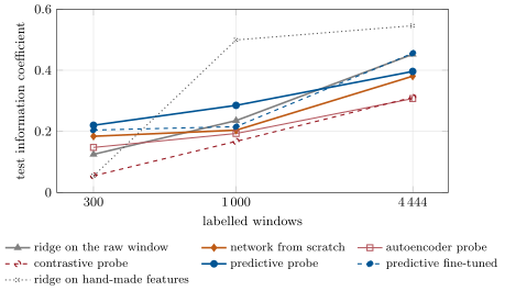Data: `ml_represent.compare`.

Figure 10.1 has one winner in the low-label regime and one lesson throughout. With 300 labelled windows (two and a half minutes of trading), the probe on the predictive encoder scores 0.22, against 0.12 for ridge on the raw window and 0.18 for the same network trained from scratch; with 1 000 windows, 0.29 against 0.24 and 0.20. With all 4 444 labelled windows, ridge on the raw window has caught up (0.45 against the probe’s 0.40), and only fine-tuning the predictive encoder keeps level with it (0.46), still ahead of the network from scratch (0.38). The reconstruction and contrastive codes do worse than the raw window at 1 000 and 4 444 labels, and at 300 the autoencoder is barely better (0.15) and the contrastive encoder worse (0.05), as Proposition 10.2 warns: they keep what varies, not what predicts.

The hand-made order-flow features of chapter 8 beat everything once there are 1 000 labels (0.50 and 0.55), and are the worst of all with 300 (0.05): ten features and a ridge regression fitted on two and a half minutes of flow that rarely moved. A label-free pre-training teaches a network what microstructure research has already written down; its value is largest where that knowledge is missing (a new market, a new data type) and the labels are few.

Method 10.7 (Pre-training on market data)

Choose a pretext close to the task: forecasting the stream’s own future beats reconstructing it for a forecast.
Pre-train on sessions disjoint from the labelled and test ones; fit normalisation on the pre-training data.
Measure with a linear probe first; fine-tune only if the probe is useful, at a small learning rate, with early stopping.
Report the learning curve in labelled data against ridge on the raw input and a network from scratch: pre-training is worth its cost only where the curves separate.

10.5 Tutorial: learning without labels

Goal. Pre-train three encoders on unlabelled sessions and measure their codes with probes and fine-tuning as the number of labels grows. End state: Figure 10.1.

The contrastive objective: two augmented views, InfoNCE over the batch.

def info_nce(z1, z2, tau: float = 0.2):
    """Symmetric InfoNCE: each view must pick its partner among the batch's 2m - 1 other views."""
    z = nn.functional.normalize(torch.cat([z1, z2]), dim=1)
    s = z @ z.T / tau
    s.fill_diagonal_(-1e9)
    m = len(z1)
    target = torch.cat([torch.arange(m, 2 * m), torch.arange(0, m)])
    return nn.functional.cross_entropy(s, target)


def pretrain_contrastive(X, code=16, hidden=(64,), noise=0.3, mask=0.2, tau=0.2, epochs=10, seed=1, batch=256,
                         lr=1e-3):
    g = _det(seed)
    enc = Encoder(X.shape[1], code, hidden)
    proj = nn.Sequential(nn.ReLU(), nn.Linear(code, code))
    opt = torch.optim.Adam(list(enc.parameters()) + list(proj.parameters()), lr=lr)
    Xt = torch.as_tensor(X, dtype=torch.float32)
    for _ in range(epochs):
        perm = torch.randperm(len(Xt), generator=g)
        for i in range(0, len(Xt) - 1, batch):
            b = Xt[perm[i:i + batch]]
            if len(b) < 2:
                continue
            opt.zero_grad()
            info_nce(proj(enc(augment(b, g, noise, mask))), proj(enc(augment(b, g, noise, mask))), tau).backward()
            opt.step()
    return enc

Listing 10.1. InfoNCE and contrastive pre-training. code/firm/represent/firm_represent.py

Self-supervised forecasting: the encoder predicts a label-free future of its input.

def pretrain_predictive(X, Y, code=16, hidden=(64,), epochs=10, seed=1, batch=256, lr=1e-3):
    """Self-supervised forecasting: the encoder, with a linear head, predicts Y -- any label-free future of the input
    (here the change of the book snapshot a few seconds later), the way a language model predicts the next word."""
    g = _det(seed)
    enc = Encoder(X.shape[1], code, hidden)
    head = nn.Linear(code, Y.shape[1])
    opt = torch.optim.Adam(list(enc.parameters()) + list(head.parameters()), lr=lr)
    Xt, Yt = torch.as_tensor(X, dtype=torch.float32), torch.as_tensor(Y, dtype=torch.float32)
    for _ in range(epochs):
        perm = torch.randperm(len(Xt), generator=g)
        for i in range(0, len(Xt), batch):
            b = perm[i:i + batch]
            opt.zero_grad()
            ((head(enc(Xt[b])) - Yt[b]) ** 2).mean().backward()
            opt.step()
    return enc

Listing 10.2. Pre-training by forecasting the stream’s own future. code/firm/represent/firm_represent.py

Run ml_represent.compare(300), compare(1000), compare(0) and fig_represent.py.

What to change next. Replace the contrastive augmentations by a time shift of one snapshot (two nearby windows as a positive pair) and see whether the codes improve; forecast the snapshot eight seconds ahead instead of two.

10.6 Build: representation learning

Purpose. Encoders pre-trained on the firm’s unlabelled market data, measured before any model is built on them.

Interface. Encoder(d_in, code, hidden), augment(x, gen, noise, mask), pretrain_dae, pretrain_contrastive, pretrain_predictive(X, Y, code, hidden, epochs, seed), info_nce(z1, z2, tau), encode(enc, X), linear_probe(Z, y, Zt, alpha), fine_tune(enc, X, y, Xv, yv, lr, epochs, patience, seed), scratch(X, y, Xv, yv, code, hidden).

Rules. Pre-training data disjoint from labelled and test data; every random draw from the run’s seed; one CPU thread.

Acceptance tests. code/firm/represent/tests/: the InfoNCE loss is $\ln(2m-1)$ for uninformative codes and near zero for identical views; a linear denoising autoencoder’s code spans the top principal subspace; the predictive encoder’s probe recovers a planted relation between a window and its future; fine-tuning does not modify the pre-trained encoder passed in.

Stretch. Masked-snapshot pre-training with a small transformer; codes pooled across several simulated instruments.

Sources and further reading

G. E. Hinton and R. R. Salakhutdinov, “Reducing the dimensionality of data with neural networks”, Science 313, 2006.
P. Vincent, H. Larochelle, Y. Bengio and P.-A. Manzagol, “Extracting and composing robust features with denoising autoencoders”, ICML, 2008.
P. Baldi and K. Hornik, “Neural networks and principal component analysis: learning from examples without local minima”, Neural Networks 2(1), 1989.
A. van den Oord, Y. Li and O. Vinyals, “Representation learning with contrastive predictive coding”, arXiv, 2018; T. Chen, S. Kornblith, M. Norouzi and G. Hinton, “A simple framework for contrastive learning of visual representations”, ICML, 2020.
Z. Yue et al., “TS2Vec: towards universal representation of time series”, AAAI, 2022.
G. Alain and Y. Bengio, “Understanding intermediate layers using linear classifier probes”, arXiv, 2016.

10.7 Exercises

Exercise 10.1 ★

A batch has $m = 256$ examples, two views each. Among how many candidates must each view find its partner under InfoNCE, and what is the loss if the encoder’s codes carry no information?

Solution

Solution of Exercise 10.1.

Among $2m - 1 = 511$ candidates; with uninformative codes every candidate is equally likely and the loss is $\ln 511 = 6.24$ .

Exercise 10.2 ★

How many labelled windows are 300 windows of half a second each, in minutes of trading? And 4 444?

Solution

Solution of Exercise 10.2.

$300\times0.5 = 150$ seconds, 2.5 minutes; $4\,444\times0.5 = 2\,222$ seconds, 37.0 minutes.

Exercise 10.3 ★

An encoder has a 400-dimensional input, 64 hidden units and a 16-dimensional code. How many parameters has it, and how many has a linear probe on its code?

Solution

Solution of Exercise 10.3.

$400\times64 + 64 + 64\times16 + 16 = 26\,704$ parameters; a linear probe on the code has $16 + 1 = 17$ .

Exercise 10.4 ★★

Why does the autoencoder’s code do worse than the raw window for the forecast, by Proposition 10.2?

Solution

Solution of Exercise 10.4.

A reconstruction objective keeps the directions of largest variance (Proposition 10.2 for the linear case), and on an order book those are the deep levels’ sizes; the top-of-book imbalance that predicts the next seconds is a small share of the variance and is partly lost in a 16-dimensional code. The raw window keeps it, and ridge can find it.

Exercise 10.5 ★★

Why does ridge on the raw window catch up with the predictive probe when the labelled data grow?

Solution

Solution of Exercise 10.5.

Ridge on 400 raw inputs has many parameters to estimate; with few labels its estimates are noisy and a 16-dimensional code that already points at the right directions wins. With 4 444 labels ridge estimates the useful directions itself, and the code’s compression starts to cost more than it saves.

Exercise 10.6 ★★

Find the flaw. “We pre-trained our encoder on all our data, including the test months, since pre-training uses no labels.”

Solution

Solution of Exercise 10.6.

Pre-training on the test months lets the encoder fit their particular states: a transductive leak that no label is needed for (distribution shift in the test period is absorbed into the representation). Pre-train only on data before the test period, as for any fitted component.

Exercise 10.7 ★★★

Coding. Pre-train the predictive encoder to forecast the snapshot’s change eight seconds ahead (AHEAD = 16) and rerun compare(1000). Does the probe improve?

Solution

Solution of Exercise 10.7.

compare(1000, ahead=16): the predictive probe falls to 0.204, from 0.285 at two seconds, level with the network from scratch. The book eight seconds ahead is mostly unpredictable, so the pretext’s target is mostly noise and the encoder learns less from it.

Exercise 10.8 ★★★

Show that the InfoNCE loss of a batch is the cross-entropy of a $(2m - 1)$ -way classification and that it equals $\ln(2m - 1)$ when all similarities are equal.

Solution

Solution of Exercise 10.8.

For view $a$ with partner $p(a)$ , the loss term is $-\ln\bigl(e^{s_{a,p(a)}}/\sum_{b\ne a}e^{s_{ab}}\bigr)$ : the cross-entropy of a softmax over the $2m - 1$ other views with the partner as the correct class. If all similarities are equal each term is $-\ln(1/(2m-1)) = \ln(2m - 1)$ , and so is their average.

10.8 Problem: Learning Without Labels

Problem 10.1

Weekend problem — three pretexts and a few labels

The chapter’s sessions: sixteen unlabelled, four labelled, one for early stopping, six for testing.

Part I — The pretexts.

What does each of the three encoders learn to do?
Which of them is closest to the task, and why?
What does Proposition 10.2 predict for the autoencoder?
What prior do the contrastive augmentations encode?

Part II — Few labels.

What do the predictive probe, ridge on the raw window and the network from scratch score with 300 labelled windows?
And with 1 000?
How do the autoencoder and contrastive probes compare?
Why are the hand-made features the worst at 300 and the best at 1 000?

Part III — Many labels.

What do the models score with all 4 444 labelled windows?
Why does fine-tuning help there while the probe does not?
What is the fine-tuned model’s gain over the network from scratch?
What would you expect with forty labelled sessions?

Part IV — The verdict.

State the named result: the labelled sample size below which pre-training helps, and the probe’s IC against the from-scratch model’s at that size.
When is pre-training worth its cost on a desk?
How would you choose augmentations for order books?
What must be kept out of the pre-training data?
How would you pre-train across instruments?
What does a linear probe tell you that fine-tuning does not?
Where does a pre-trained language model fit in this picture (chapter 14)?
In one sentence: what makes a pretext useful?

Solution

Solution of Problem 10.1.

Reconstruct a masked, noisy window; match two augmented views of a window against other windows; forecast the change of the book two seconds after the window.
The forecasting pretext: its target is the stream’s own near future, the same kind of object as the task’s.
That its code keeps the directions of largest variance, which need not be predictive.
That Gaussian noise and random masking of entries do not change what matters about a window.
0.22, 0.12 and 0.18.
0.29, 0.24 and 0.20.
Worse than the raw window at 1 000 and 4 444; at 300 the autoencoder 0.15, the contrastive encoder 0.05.
Ten features fitted on two and a half minutes of mostly flat flow are noise; with more data they carry the microstructure knowledge the networks must learn.
Ridge on the raw window 0.45, the predictive probe 0.40, fine-tuned 0.46, from scratch 0.38, the autoencoder and contrastive probes 0.31, the hand-made features 0.55.
Fine-tuning adapts the encoder’s code to the task once there are enough labels to do so safely; a frozen code keeps only what the pretext kept.
$0.46 - 0.38 = 0.08$ of IC.
The curves to converge: with many labels, pre-training’s advantage fades and ridge on raw or hand-made inputs catch up.
Named result: below about 1 000 labelled windows (eight minutes) the predictive probe beats every raw-input model trained on labels alone: 0.22 against 0.18 from scratch at 300, 0.29 against 0.20 at 1 000; with 4 444 only the fine-tuned encoder keeps level with ridge.
When labels are scarce and unlabelled data plentiful, and when no one has written down the features (a new market, a new data type).
From what should not change a forecast: small measurement noise, shifts by a snapshot, rescaling of deep levels; test them with a probe, not by taste.
The test period and anything after it.
Pool sessions of many instruments, with per-instrument normalisation, and probe on each.
How much of the task is linearly available in the representation, independently of how a downstream model is trained.
It is a very large self-supervised forecaster of text, used through probes, prompts or fine-tuning.
Being close to the task, so that what it keeps is what the task needs.

10.9 Interview questions

Interview question 10.1 ★ mle

What is the difference between a linear probe and fine-tuning, and when do you use each?

Solution

Solution of Interview question 10.1.

A linear probe fits a linear model on frozen codes: cheap, measures what the representation holds, safe with few labels. Fine-tuning trains the encoder too: can adapt the representation, needs more labels and care (small learning rate, early stopping). Probe first; fine-tune when there are enough labels.

What the interviewer is looking for: the trade-off between adaptation and overfitting.

Interview question 10.2 ★★ mle, researcher

Explain contrastive learning. What would you use as augmentations for intraday price data?

Solution

Solution of Interview question 10.2.

Train codes so that two views of one example are close and views of different examples far (InfoNCE). For intraday prices: small noise, small time shifts, masking of some features, rescaling of volumes; never transformations that change direction or future outcome (reversing time, flipping sides).

What the interviewer is looking for: the objective and augmentations that respect what matters.

Interview question 10.3 ★★ researcher

You have ten years of unlabelled tick data and three months of labels for a new strategy. How do you use the ten years?

Solution

Solution of Interview question 10.3.

Pre-train an encoder on the ten years with a self-supervised pretext close to the task (forecasting the next seconds or days of the stream), then probe and possibly fine-tune on the three months; compare on held-out labelled data with a model trained from scratch.

What the interviewer is looking for: a pretext aligned with the task and an honest comparison.

Interview question 10.4 ★★ researcher, mle

Why can an autoencoder’s code be useless for prediction although it reconstructs the input well?

Solution

Solution of Interview question 10.4.

It keeps what varies most in the input (PCA for a linear autoencoder), and the predictive part of the input may be a low-variance direction the code drops.

What the interviewer is looking for: variance is not relevance.

Interview question 10.5 ★★ mle

How do you evaluate a pre-trained representation without committing to a downstream model?

Solution

Solution of Interview question 10.5.

Linear probes on held-out data for several tasks, and the learning curve in labelled data against a raw-input baseline.

What the interviewer is looking for: probes and learning curves.

Interview question 10.6 ★★★ researcher

Prove that the best linear autoencoder with a $k$ -dimensional code projects onto the first $k$ principal components.

Solution

Solution of Interview question 10.6.

The reconstruction $BAX$ has rank at most $k$ ; by Eckart–Young the best rank- $k$ Frobenius approximation of $X$ is the truncated SVD, i.e. the projection onto the top $k$ right singular vectors, the principal directions; choosing $A$ as the projection’s coordinates and $B$ as its basis attains it.

What the interviewer is looking for: the rank argument and Eckart–Young.

Terms defined in this chapter

See all 2333 terms in the glossary