Machine Learning for Markets · Machine learning
11Probabilistic Models and Uncertainty
Two forecasts both say a stock will rise five basis points tomorrow. One comes with a standard deviation of 80 basis points, the other with 250: the same expected return on a quiet day and on a violent one. A book that sizes the two trades alike holds three times the risk per unit of expected return in the second, and a risk report that shows only the point forecast cannot tell them apart. Every forecast of a return is a distribution. This chapter trains models that say so, scores them with losses that reward honest distributions, builds intervals whose coverage survives a change of regime, and measures what the variance is worth when positions are sized.
11.1 Predictive distributions and proper scoring rules
Definition 11.1 (Predictive distribution, proper scoring rule)
A predictive distribution is a forecast of the whole conditional distribution of the target. A scoring rule gives a loss to a forecast when occurs; it is a proper scoring rule if its expected value under the true distribution is minimised by forecasting , so that honesty is optimal (Gneiting and Raftery, 2007). The negative log-likelihood is proper; so are the two rules below.
Definition 11.2 (Pinball loss, continuous ranked probability score)
The pinball loss of a forecast of the -quantile is . The continuous ranked probability score of a forecast distribution is , in the units of the target; for a Gaussian forecast it has a closed form.
Proposition 11.3 (The pinball loss elicits the quantile)
If has a continuous distribution function , is minimised at .
Proof. , which is zero at , negative before and positive after. ∎
The chapter’s data are firm.mlsynth’s daily series: twenty assets, ten years, GARCH volatility, Student- shocks with five degrees of freedom, a planted drift, and a regime from day 2 100 in which every shock is 1.6 times larger. The target is the next day’s return; the features are the drift reading, the 5- and 20-day returns, the ratio of short to long realised volatility and an EWMA volatility, all known at the close. Training days 60–1 511, calibration days 1 512–1 763, test days 1 764–2 518: the regime changes about half-way through the test.
11.2 Quantile and distributional losses
Definition 11.4 (Quantile regression, mixture density network)
Quantile regression fits the conditional -quantile by minimising the average pinball loss (Koenker and Bassett, 1978); with several levels it describes the whole distribution. A mixture density network outputs the weights, means and standard deviations of a mixture of Gaussians and is trained by their negative log-likelihood (Bishop, 1994).
Three distributional models are fitted: gradient-boosted trees for nineteen quantile levels (5% to 95%), a network with a mean and a log-variance output trained by the Gaussian negative log-likelihood (five seeds, averaged as a deep ensemble, chapter 7), and a two-component mixture density network. Table 11.1 scores them with the CRPS on the nineteen quantiles and the coverage of their 90% intervals, before and after the regime change, beside the true conditional distribution’s Gaussian approximation.
| before day 2 100 | after day 2 100 | |||
| model | CRPS (bp) | 90% coverage | CRPS (bp) | 90% coverage |
| boosted quantiles | 78.9 | 89.4% | 136.3 | 85.0% |
| Gaussian network (one seed) | 79.0 | 90.6% | 135.3 | 87.0% |
| ensemble of five | 79.1 | 91.1% | 135.4 | 87.6% |
| mixture density network | 78.8 | 89.7% | 136.1 | 86.1% |
| truth (Gaussian approximation) | 78.9 | 91.2% | 135.5 | 91.3% |
ml_uncert.scores.Before the break the four models are as good as the truth’s approximation, within a quarter of a basis point of CRPS: the volatility they must forecast is persistent and the EWMA feature carries most of it. After the break the CRPS of all of them nearly doubles, as the truth’s does, but their intervals cover 85–88% of the days instead of 90%: the features adapt with a lag and the models were fitted on a calmer world. The mean forecasts are another matter; a signal-to-noise ratio of a few hundredths hardly moves any of these scores, which are dominated by the volatility.
11.3 Two kinds of uncertainty
Definition 11.5 (Aleatoric and epistemic uncertainty)
Aleatoric uncertainty is the randomness of the target given the inputs, which more data cannot remove; epistemic uncertainty is the model’s uncertainty about the function itself, which more data reduce. In a deep ensemble the average of the members’ predicted variances estimates the first and the variance of their means the second; the predictive variance is their sum.
On the chapter’s test days the epistemic part is 0.09% of the predictive variance. Daily returns are almost all aleatoric: nothing a model learns will narrow them much. The epistemic part matters where the model is extrapolating (inputs outside the training range, a new instrument) and in the few-label settings of chapter 10; it is the part an ensemble, not a single network, can report (Kendall and Gal, 2017).
11.4 Conformal prediction
Definition 11.6 (Conformal prediction)
Conformal prediction turns any forecast into prediction sets with a coverage guarantee: a score (for example , or that divided by a predicted standard deviation) is computed on calibration examples, and the set for a new is with the -th smallest calibration score (split conformal; Vovk, Gammerman and Shafer, 2005). The adaptive version updates the level online, , to keep the long-run error rate at when the data drift (Gibbs and Candès, 2021).
Theorem 11.7 (Split conformal coverage)
If the calibration scores and the new score are exchangeable, .
Proof. By exchangeability the rank of among the scores is uniform on (ties broken at random). whenever its rank is at most , which has probability . ∎
Exchangeability is exactly what a regime change breaks (Figure 11.1). Around the boosted trees’ mean forecast, split conformal on the calibration year covers 90.7% of the test days before the break and 74.0% after it, with a fixed width. Dividing the score by the ensemble’s predicted standard deviation lets the width follow volatility: 90.3% before, 86.9% after. Adaptive conformal on the same normalised scores, updated day by day through the test period with , covers 89.9% before and 90.1% after (Figure 11.2): it gives up the finite-sample guarantee for a long-run one that survives drift.
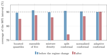
ml_uncert.scores and ml_uncert.conformal.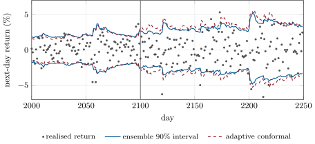
ml_uncert.conformal.11.5 Using uncertainty in sizing
For independent bets, the weight that maximises the Sharpe ratio of their sum is proportional to the expected return over the variance; Kelly sizing (Book 2, chapter 29) has the same form. The variance is where the model’s distribution earns its keep. The chapter’s sizing test must be longer than its three test years, because Sharpe ratios estimated on three years differ by more than the effect: on twenty-year series of twenty assets (four seeds, scored after the first seven years), a daily portfolio weighted by the drift reading alone earns an annualised Sharpe ratio of 1.72 on average; dividing the reading by a variance forecast raises it to 1.90 with the EWMA variance, 1.91 with the Gaussian network’s predicted variance and 1.93 with the true variance. With the true mean the gain is larger (2.94 to 3.31): the better the mean forecast, the more the variance matters.
Method 11.8 (Forecasting and using a distribution)
- Train with a proper score (negative log-likelihood, pinball losses) and evaluate with another (CRPS) and with coverage, on held-out periods including a stressed one.
- Use an ensemble to separate epistemic from aleatoric variance; report both.
- Wrap the forecast in conformal intervals, normalised by the predicted scale, and update them online.
- Size by the mean over the variance, and test the rule on samples long enough for Sharpe ratios to differ.
11.6 Tutorial: sizing by doubt
Goal. Fit quantile, Gaussian and mixture models of the next day’s return, score them before and after a volatility regime, build split and adaptive conformal intervals, and size positions by the predicted variance. End state: Table 11.1, Figures 11.1 and 11.2, the sizing numbers.
Scores: pinball, CRPS on a quantile grid, coverage.
def pinball(y, q, alpha):
    d = np.asarray(y) - np.asarray(q)
    return float(np.mean(np.maximum(alpha * d, (alpha - 1) * d)))


def crps_gaussian(y, mu, sigma):
    from scipy.stats import norm

    z = (np.asarray(y) - mu) / sigma
    return float(np.mean(sigma * (z * (2 * norm.cdf(z) - 1) + 2 * norm.pdf(z) - 1 / math.sqrt(math.pi))))


def crps_quantiles(y, Q, alphas):
    return 2.0 * float(np.mean([pinball(y, Q[:, j], a) for j, a in enumerate(alphas)]))


def coverage(y, lo, hi):
    y = np.asarray(y)
    return float(np.mean((y >= lo) & (y <= hi)))
Listing 11.1. The pinball loss, the CRPS and coverage. code/firm/uncert/firm_uncert.py Conformal: the split threshold and the adaptive online level.
def split_conformal(scores, alpha):
    s = np.sort(np.asarray(scores))
    n = len(s)
    k = min(n, math.ceil((n + 1) * (1 - alpha)))
    return float(s[k - 1])


def adaptive_conformal(scores, alpha, gamma=0.005, window=500, start=None):
    """Online conformal thresholds: at each step t the threshold is the (1 - alpha_t) quantile of the last `window`
    scores; after seeing whether score t exceeded it, alpha_{t+1} = alpha_t + gamma (alpha - err_t)."""
    scores = np.asarray(scores)
    a = alpha
    th, err = np.empty(len(scores)), np.empty(len(scores))
    hist = list(start) if start is not None else []
    for t, s in enumerate(scores):
        pool = np.asarray(hist[-window:])
        q = np.quantile(pool, min(max(1 - a, 0.0), 1.0)) if len(pool) else np.inf
        th[t] = q
        err[t] = float(s > q)
        a = a + gamma * (alpha - err[t])
        hist.append(s)
    return th, err
Listing 11.2. Split and adaptive conformal prediction. code/firm/uncert/firm_uncert.py - Run
ml_uncert.scores(),conformal(),sizing()andfig_uncert.py.
What to change next. Raise to 0.02 and watch adaptive coverage recover faster and wobble more; size by the mean over the standard deviation instead of the variance.
11.7 Build: predictive distributions and intervals
Purpose. Every forecast the firm uses comes with a distribution, a score for it, and an interval that holds up.
Interface. pinball, crps_gaussian, crps_quantiles, coverage; GaussNet, MDN, fit_nll, predict_gauss, predict_mdn, mdn_quantile; ensemble_split; split_conformal(scores, alpha), adaptive_conformal(scores, alpha, gamma, window, start).
Rules. Calibration data disjoint from training data and before the test; adaptive thresholds use only past scores; every network deterministic on one thread.
Acceptance tests. code/firm/uncert/tests/: the pinball loss is minimised at the empirical quantile; the Gaussian CRPS matches the quantile-grid approximation; split conformal covers at least on exchangeable data across many draws; adaptive conformal restores coverage after a planted scale change; the Gaussian network and the mixture recover a planted heteroskedastic and a bimodal distribution.
Stretch. Conformalised quantile regression; conformal sets for classifiers (chapter 2’s labels); a sizing rule that shrinks the variance forecast.
Sources and further reading
- T. Gneiting and A. E. Raftery, “Strictly proper scoring rules, prediction, and estimation”, Journal of the American Statistical Association 102(477), 2007.
- R. Koenker and G. Bassett, “Regression quantiles”, Econometrica 46(1), 1978.
- C. M. Bishop, “Mixture density networks”, Aston University technical report NCRG/94/004, 1994.
- V. Vovk, A. Gammerman and G. Shafer, Algorithmic Learning in a Random World, Springer, 2005; 2nd ed., 2022.
- I. Gibbs and E. Candès, “Adaptive conformal inference under distribution shift”, NeurIPS, 2021.
- A. Kendall and Y. Gal, “What uncertainties do we need in Bayesian deep learning for computer vision?”, NeurIPS, 2017.
11.8 Exercises
Exercise 11.1 ★
A 95% quantile forecast is 2.0%; the return is 3.0%. What is the pinball loss? And if the return is 1.0%?
Solution
Solution of Exercise 11.1.
: loss . With , : loss . The asymmetry is what makes the minimiser the 95% quantile.
Exercise 11.2 ★
With 250 calibration scores and , which order statistic is the split conformal threshold? With 5 040?
Solution
Solution of Exercise 11.2.
th smallest of 250; th of 5 040.
Exercise 11.3 ★
Two bets have expected returns of 5 basis points and standard deviations of 80 and 250 basis points. In what proportion should mean-variance sizing hold them?
Solution
Solution of Exercise 11.3.
Weights : .
Exercise 11.4 ★★
Why does the raw split conformal interval lose so much coverage after the break, and the normalised one less?
Solution
Solution of Exercise 11.4.
The raw interval has a fixed width set on the calm calibration year; when every shock is 1.6 times larger the same width covers far fewer returns (74.0%). The normalised score divides by the predicted scale, which rises with the EWMA volatility after the break, so the width follows the new regime, with a lag (86.9%).
Exercise 11.5 ★★
The epistemic part of the predictive variance is 0.09%. What does that say about the value of more data for this forecast, and where would you expect it to be larger?
Solution
Solution of Exercise 11.5.
Almost all the predictive variance is the return’s own randomness; more data would narrow the forecast very little. The epistemic part is larger where the model extrapolates: inputs outside the training range, new instruments, small samples.
Exercise 11.6 ★★
Find the flaw. “Sizing by the predicted variance lowered our Sharpe ratio from 2.1 to 1.8 over our three-year test, so variance scaling does not work for this signal.”
Solution
Solution of Exercise 11.6.
The standard error of an annualised Sharpe ratio over three years is about ; a difference of 0.3 is noise. On twenty-year samples and four seeds the same rule raises the Sharpe ratio (1.72 to 1.91). Test sizing rules on long samples or many seeds.
Exercise 11.7 ★★★
Coding. Run the adaptive conformal intervals of ml_uncert.conformal with . Report the coverage after the break and explain the trade-off.
Solution
Solution of Exercise 11.7.
conformal(gamma=0.02): coverage after the break 90.0% (90.1% with ). A larger reacts faster to a run of misses but moves the threshold more from day to day, widening and narrowing the band on noise; a smaller one is smoother and slower after a break.
Exercise 11.8 ★★★
Show that the CRPS equals twice the integral over of the pinball loss of the forecast’s -quantile.
Solution
Solution of Exercise 11.8.
. Substituting , , and integrating by parts, (Gneiting and Raftery, 2007, give the identity).
11.9 Problem: Sizing by Doubt
Problem 11.1
Weekend problem — distributions through a regime change
The chapter’s twenty assets, the volatility regime from day 2 100, and the four ways of forecasting the next day.
Part I — Scores.
- Why must a score be proper, and which of the chapter’s scores are?
- What do the models score (CRPS and coverage) before the break?
- And after it?
- Why are the CRPS so close across models and the truth?
Part II — Uncertainty.
- What share of the predictive variance is epistemic?
- What does a deep ensemble add to a single Gaussian network here?
- What does the mixture density network model that the Gaussian network does not?
- Where would you expect the epistemic share to matter?
Part III — Conformal.
- What do split conformal intervals cover before and after the break, raw and normalised?
- What does adaptive conformal cover, and what does it give up?
- Which assumption does the break violate?
- How would you choose ?
Part IV — Sizing and the verdict.
- Why is the sizing test run on twenty-year series?
- What Sharpe ratios do the four rules earn with the drift reading, and with the true mean?
- Why does the variance matter more with a better mean forecast?
- State the named result: the Sharpe gain of variance-scaled sizing over sizing by the mean alone, and conformal coverage against its nominal 90% after the regime change.
- What should a risk report show beside a point forecast?
- How would you monitor a model’s intervals in production (chapter 27)?
- What would change with a fat-tailed target and a Gaussian model?
- In one sentence: what is a forecast of a return?
Solution
Solution of Problem 11.1.
- A proper score’s expectation is minimised by the true distribution, so no forecaster gains by shading; the log-likelihood, the pinball loss and the CRPS are proper.
- CRPS 78.8–79.1 basis points for all, coverage 89.4–91.1%.
- CRPS 135.3–136.3, coverage 85.0–87.6% (the truth 91.3%).
- The score is dominated by the volatility, which all of them forecast from the same persistent features; the mean forecast’s signal is a few hundredths of the variance.
- 0.09%.
- The split into aleatoric and epistemic variance, and a slightly better calibrated interval (91.1% and 87.6% against 90.6% and 87.0% for one seed).
- Skewness and fat tails through two components (here with coverage 89.7% and 86.1%).
- Out of the training range, for new instruments, and with few labels.
- Raw: 90.7% and 74.0%; normalised: 90.3% and 86.9%.
- 89.9% and 90.1%; it gives up the finite-sample guarantee for a long-run error rate under drift.
- Exchangeability of calibration and test scores.
- From the speed of the drifts expected and the tolerance for a wobbling width: small (0.005) for slow changes.
- Over three years Sharpe ratios have a standard error near 0.6, larger than the effect.
- Reading 1.72; over the EWMA variance 1.90, over the network’s 1.91, over the true 1.93. True mean 2.94, over the true variance 3.31.
- Scaling reweights the signal’s expected profits; the more of the mean is signal rather than noise, the more there is to reweight.
- Named result: dividing the drift reading by the network’s predicted variance raises the Sharpe ratio from 1.72 to 1.91 (1.93 with the true variance); after the regime change split conformal intervals cover 74.0% (raw) or 86.9% (normalised) of the nominal 90%, adaptive conformal 90.1%.
- The predictive standard deviation or an interval, and its recent coverage.
- Track the interval’s hit rate and the normalised errors’ distribution with the drift detectors of chapter 12 and the alarms of chapter 27.
- Too-narrow tails: a Gaussian model under-covers extremes; use quantiles, a mixture, or conformal intervals.
- A distribution, of which the point forecast is one summary.
11.10 Interview questions
Interview question 11.1 ★ researcher, mle
What is a proper scoring rule, and why should you train and evaluate forecasts with one?
Solution
Solution of Interview question 11.1.
A score whose expected value is minimised by forecasting the true distribution. Training with it makes honest distributions the optimum; evaluating with it lets different forecasts be compared without rewarding over- or under-confidence.
What the interviewer is looking for: the definition and the incentive argument.
Interview question 11.2 ★★ mle
How would you get prediction intervals out of a gradient-boosted model?
Solution
Solution of Interview question 11.2.
Fit quantile objectives (pinball loss) at the interval’s levels, or a mean model plus a model of the absolute residual, and wrap either in conformal calibration on held-out data (conformalised quantile regression).
What the interviewer is looking for: quantile losses and calibration on held-out data.
Interview question 11.3 ★★ researcher
Explain split conformal prediction and its guarantee. When does the guarantee fail in trading?
Solution
Solution of Interview question 11.3.
Compute scores on a calibration set; the threshold is their -th smallest; intervals are the values whose score is below it; coverage is at least if calibration and new scores are exchangeable. It fails when markets change regime (volatility, liquidity), since the calibration scores no longer describe the new ones; use normalised scores and adaptive updates.
What the interviewer is looking for: the construction, the exchangeability condition, and the remedy.
Interview question 11.4 ★★ researcher, trader
Your model forecasts both the mean and the variance of tomorrow’s return. How do you size positions, and how would you test the rule?
Solution
Solution of Interview question 11.4.
In proportion to the mean over the variance (Kelly or mean-variance), possibly shrunk; test on long histories or many simulated paths, since the Sharpe ratio differences between rules are small relative to their standard errors.
What the interviewer is looking for: mean over variance, and a test with enough power.
Interview question 11.5 ★★ mle, researcher
What is the difference between aleatoric and epistemic uncertainty, and how do you estimate each?
Solution
Solution of Interview question 11.5.
Aleatoric: the target’s noise given the inputs, estimated by a predicted variance. Epistemic: uncertainty about the model, estimated by the disagreement of an ensemble (or a posterior). The first stays with more data, the second shrinks.
What the interviewer is looking for: the definitions and an estimator for each.
Interview question 11.6 ★★★ researcher
Prove that the expected pinball loss is minimised by the true quantile.
Solution
Solution of Interview question 11.6.
for continuous : negative below the -quantile, positive above, so the minimum is at .
What the interviewer is looking for: the derivative and the sign argument.