Machine Learning for Markets · Machine learning

4Linear and Regularised Baselines

A team spends a quarter on gradient-boosted trees for the cross-section of 500 stocks. Out of sample, over ten years, their long-short decile portfolio earns a Sharpe ratio of 1.90 after costs. A lasso regression on the same forty ranked characteristics, with its penalty chosen by cross-validation, is fitted in a second and earns 1.91. The trees forecast better (an out-of-sample R-squared of 0.47% against 0.32%), and on a portfolio that trades the extremes of the ranking the difference is gone. This chapter builds the model every later model must beat, and measures when and why it is hard to beat.

4.1 The model to beat

Definition 4.1 (Baseline model)

A baseline model is the simplest credible model of a task, fitted and evaluated with the same data, splits, target and report as the candidate: any claim that a model works is a claim that it beats the baseline by more than the noise of the comparison.

The baseline is a discipline, not a formality. It catches the leaks of chapter 3 (a baseline that scores as well as the candidate on a target that should be hard points at the pipeline), it prices complexity, and it is the model that runs in production while the candidate is being validated. firm.mlbase is the harness every cross-sectional model of the book goes through: features ranked by date, the target demeaned by date (chapter 1), a fit on the training months, and one report for the test months: R-squared against zero, the mean rank information coefficient with its HAC $t$ (Book 7, chapter 6), and the Sharpe ratio of an equal-weighted long-short decile portfolio, gross and net of 20 basis points per unit traded.

The chapter’s panel is firm.mlsynth’s with forty characteristics, six of them carrying a planted expected return (half of its variance nonlinear), and one addition that matters: every characteristic also carries a factor return of zero mean and 2% monthly volatility. A portfolio sorted on characteristics then carries factor risk, as real ones do, and its Sharpe ratio comes down to the published range: Gu, Kelly and Xiu’s equal-weighted decile portfolios reach 2.45 for their best network and 0.83 for a three-variable linear model. Without the factor returns the same models would report Sharpe ratios near 5.

4.2 Regularised regression on ranked features

Ordinary least squares, ridge regression, the lasso and the elastic net are Book 4’s (chapter 16). What this chapter adds is how their penalty is chosen and what the choice looks like on market data.

Definition 4.2 (Regularisation path)

The regularisation path of a penalised estimator is its solution, or its validation score, as a function of the penalty $\lambda$ ; the penalty is chosen at the path’s best purged cross-validated score.

Regularisation paths: pooled out-of-fold R-squared of three purged folds of the twenty training years, as a function of the penalty. Ridge peaks at = 104 (training folds of about 80 000 rows), the lasso at 10-3; one step further the lasso sets every coefficient to zero and scores zero. Data: ml_baselines.paths. — **Figure 4.1.** Regularisation paths: pooled out-of-fold R-squared of three purged folds of the twenty training years, as a function of the penalty. Ridge peaks at $\lambda = 10^4$ (training folds of about 80 000 rows), the lasso at $10^{-3}$ ; one step further the lasso sets every coefficient to zero and scores zero. 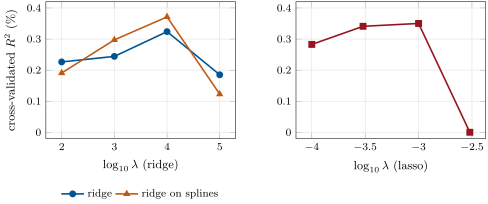Data: `ml_baselines.paths`.

The paths are flat near their peaks and fall steeply on either side (Figure 4.1). At its peak the lasso keeps six coefficients; one step further it keeps none, and a model that predicts zero everywhere scores zero, which is better than any of the unpenalised fits on the left of the figure. Least squares on 120 000 rows and forty features looks like a well-determined problem; with the factor returns making the months, not the rows, the effective sample (chapter 1), it is not, and the penalty that wins is large.

Method 4.3 (Choosing a penalty on a panel)

Rank each feature by date; demean the target by date.
Build purged folds of whole dates (a date’s rows never straddle folds), with an embargo of the label length.
Evaluate a logarithmic grid wide enough that both ends are worse than the middle; if the best value is at an end, extend the grid.
Prefer the most penalised value within one standard error of the best (the path’s plateau, not its peak).

4.3 Dimension reduction: principal-component and partial least squares

Definition 4.4 (Principal component regression, partial least squares)

Principal component regression (PCR) regresses the target on the first $k$ principal components of the features (Book 4, chapter 22). Partial least squares (PLS) regresses it on $k$ components chosen for their covariance with the target: the first weight vector is proportional to $X^\top y$ , and each later one is found the same way after deflating $X$ by the components already taken.

Proposition 4.5 (What each reduction keeps)

Among unit vectors $w$ , $w\propto X^\top y$ maximises the sample covariance of $Xw$ with $y$ , whereas the first principal direction maximises the variance of $Xw$ whatever $y$ is. When the features are uncorrelated with equal variance, every direction has the same variance and the principal components are arbitrary; PLS’s first component is the least-squares fit’s direction up to scale.

Proof. $\widehat{\Cov}(Xw, y)\propto w^\top X^\top y \le \lVert w\rVert\,\lVert X^\top y\rVert$ by Cauchy–Schwarz, with equality for $w\propto X^\top y$ . If $X^\top X = cI$ , the sample variance $w^\top X^\top Xw/n = c/n$ is the same for every unit $w$ ; the least-squares coefficient is $(X^\top X)^{-1}X^\top y = X^\top y/c$ . ∎

Cross-sectional ranks are close to that case: forty characteristics of equal variance and little correlation. PCR needs ten components before it recovers the signal and still scores only 0.13%; PLS’s single component already does what least squares does, and the two score alike (Table 4.1). On real characteristics, which are correlated in blocks (value measures with each other, momentum measures with each other), PCR does better, and Gu, Kelly and Xiu found PCR and PLS at 0.26% and 0.27%, above their elastic net’s 0.11%.

4.4 Classification baselines

Definition 4.6 (Logistic regression)

Logistic regression models $\P(y = 1\mid x) = 1/(1 + e^{-(b + x^\top\beta)})$ and fits $(b,\beta)$ by maximum likelihood, usually with a ridge or lasso penalty on $\beta$ .

Labels that are signs (chapter 2) call for a classifier; its natural baseline is the logistic regression. On the panel it ranks stocks as well as the regressions do (IC 0.060, as for ridge) with a probability to spare: throwing away the size of each return costs almost nothing when that size is mostly noise.

Definition 4.7 (Basis expansion)

A basis expansion replaces each feature $x_j$ by functions $h_{j1}(x_j),\dots,h_{jm}(x_j)$ (splines, indicators of bins, polynomials) and fits a linear model on them; the model is additive in the features and nonlinear in each.

Ridge regression on quadratic splines with four knots per characteristic is the strongest linear baseline of the panel (R-squared 0.35%): it captures the square and the absolute value the truth contains, but not the interaction, which no additive model can.

model (parameter)	$R^2_{\mathrm{oos}}$	IC	$t$ (HAC)	Sharpe gross	Sharpe net	turnover
ordinary least squares	0.25%	0.060	5.6	1.85	1.61	0.83
ridge ( $\lambda = 10^4$ )	0.30%	0.060	5.6	1.83	1.59	0.83
lasso ( $\lambda = 10^{-3}$ )	0.32%	0.066	6.7	2.17	1.91	0.80
elastic net	0.32%	0.066	6.7	2.17	1.91	0.80
PCR (10 components)	0.13%	0.043	4.1	1.23	0.99	0.77
PLS (1 component)	0.25%	0.061	5.6	1.87	1.62	0.82
logistic regression	0.22%	0.060	5.7	1.84	1.59	0.84
ridge on splines	0.35%	0.064	6.2	1.98	1.69	0.95
boosted trees	0.47%	0.076	7.8	2.20	1.90	0.97
ceiling	0.71%

Table 4.1. Ten test years of the forty-characteristic panel with factor risk (500 stocks, twenty training years). Sharpe ratios of the equal-weighted top-minus-bottom decile portfolio, annualised, net of 20 basis points per unit traded; turnover is the share of the gross book traded each month. Data: ml_baselines.table.

4.5 Why the baseline often wins

Table 4.1 ranks the models by R-squared, and the ranking by net Sharpe ratio is not the same. The boosted trees forecast best (0.47% against the lasso’s 0.32%), but their predictions change more from month to month (turnover 0.97 against 0.80), their portfolio pays more in costs, and at the extremes of the ranking, where a decile portfolio trades, the two models mostly agree. The lasso’s net Sharpe ratio of 1.91 ties the trees’ 1.90.

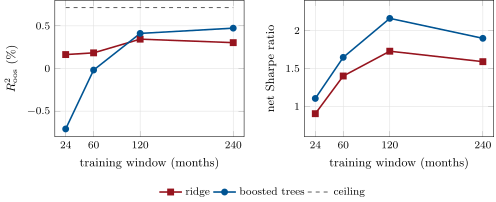
The comparison also depends on how much history there is (Figure 4.2). Trained on the last two years before the test, the trees’ R-squared is $-0.71\%$ , although their decile portfolio still earns a Sharpe ratio of 1.11 against ridge’s 0.90: with little data the trees rank stocks tolerably and size their forecasts badly, which is the difference between the IC and R-squared (Proposition 1.6). They overtake ridge in R-squared between five and ten years of history. On real data the argument has a second half: Kelly, Malamud and Zhou show that heavily regularised models with more parameters than observations can predict better than small ones, so “simple” is not the claim; “regularised, and compared on equal terms” is.

Ridge and boosted trees trained on the last 2 to 20 years before the same ten test years. Left, R-squared against zero; right, the net Sharpe ratio of the decile portfolio. The trees’ ranking is useful early; their sizes are not. Data: ml_baselines.crossing. — **Figure 4.2.** Ridge and boosted trees trained on the last 2 to 20 years before the same ten test years. Left, R-squared against zero; right, the net Sharpe ratio of the decile portfolio. The trees’ ranking is useful early; their sizes are not. Data: `ml_baselines.crossing`.

4.6 Tutorial: the model to beat

Goal. Fit the linear baselines along their regularisation paths through firm.mlbase, compare them with boosted trees on one report, and vary the training window. End state: Table 4.1, Figures 4.1 and 4.2.

The report: R-squared against zero, the rank IC with its HAC $t$ , and the decile portfolio gross and net.

def long_short(pred, r, q: int = 10):
    m, n = pred.shape
    k = max(1, n // q)
    order = np.argsort(pred, axis=1)
    w = np.zeros((m, n))
    rows = np.arange(m)[:, None]
    w[rows, order[:, -k:]] = 1.0 / k
    w[rows, order[:, :k]] = -1.0 / k
    return (w * r).sum(axis=1), w


def report(pred, r, q: int = 10, cost_bp: float = 20.0, periods: int = 12) -> dict:
    ic = ic_series(pred, r, "rank")
    s = ic_summary(ic, h=1, periods=periods)
    ls, w = long_short(pred, r, q)
    traded = np.r_[np.abs(w[0]).sum(), np.abs(np.diff(w, axis=0)).sum(axis=1)]   # per unit of capital (gross 2)
    net = ls - traded * cost_bp * 1e-4
    turn = traded / np.abs(w).sum(axis=1)                              # share of the gross book traded
    sr = float(ls.mean() / ls.std() * math.sqrt(periods))
    return {"r2": r2_oos(r, pred), "ic": float(s["mean"]), "ic_t": float(s["t_hac"]), "ls_sr": sr,
            "ls_sr_net": float(net.mean() / net.std() * math.sqrt(periods)), "turnover": float(turn.mean())}

Listing 4.1. The long-short decile portfolio and the standard report. code/firm/mlbase/firm_mlbase.py

The path: purged folds of whole months, pooled out-of-fold R-squared.

def cv_path(make, params, X, r, months, n_folds: int = 5, embargo: int = 1):
    """Purged k-fold over months (a label spans one period), pooled out-of-fold R-squared against zero."""
    months = np.asarray(months)
    folds = purged_kfold(months, months, n_folds, embargo)
    scores = []
    for p in params:
        pred = np.full((len(months), X.shape[1]), np.nan)
        for tr, te in folds:
            m = fit(make(p), X, r, months[tr])
            pred[te] = predict(m, X, months[te])
        scores.append(r2_oos(r[months], pred))
    return list(params), np.array(scores)

Listing 4.2. Cross-validated regularisation path. code/firm/mlbase/firm_mlbase.py

Run ml_baselines.paths(), table(), crossing() and fig_baselines.py.

What to change next. Set the factor volatility to zero and watch every Sharpe ratio double; add the interaction $c_0c_3$ as a feature to ridge on splines and see how much of the trees’ advantage it removes.

4.7 Build: the model harness

Purpose. Every cross-sectional model is compared with the same baselines, on the same splits, with the same report.

Interface. rank_features(X), xs_target(r, months), fit(model, X, r, months, target), predict(model, X, months), long_short(pred, r, q), report(pred, r, q, cost_bp, periods) returning r2, ic, ic_t, ls_sr, ls_sr_net, turnover; cv_path(make, params, X, r, months, n_folds, embargo); Harness(make, target).run(X, r, train, test).

Rules. Any scikit-learn-style regressor plugs in; folds are whole dates; the report is computed on test dates only; costs are charged on traded notional.

Acceptance tests. code/firm/mlbase/tests/: ranks and demeaned targets; decile weights that sum to zero with gross two; the harness finds a planted signal and reports gross above net; the path prefers a moderate penalty on noisy data.

Stretch. Value-weighted deciles; the report by size group; a random-feature ridge in the spirit of Kelly, Malamud and Zhou as a further baseline.

Sources and further reading

S. Gu, B. Kelly and D. Xiu, “Empirical asset pricing via machine learning”, Review of Financial Studies 33(5), 2020.
I. Welch and A. Goyal, “A comprehensive look at the empirical performance of equity premium prediction”, Review of Financial Studies 21(4), 2008.
B. Kelly, S. Malamud and K. Zhou, “The virtue of complexity in return prediction”, Journal of Finance 79(1), 2024.
S. de Jong, “SIMPLS: an alternative approach to partial least squares regression”, Chemometrics and Intelligent Laboratory Systems 18, 1993.
A. E. Hoerl and R. W. Kennard, “Ridge regression: biased estimation for nonorthogonal problems”, Technometrics 12(1), 1970.

4.8 Exercises

Exercise 4.1 ★

A decile portfolio of 500 stocks holds 50 long and 50 short, equally weighted, gross 2. In a month 30 names change on each side. What share of the gross book is traded, and what does it cost at 20 basis points per unit traded?

Solution

Solution of Exercise 4.1.

Each side sells 30 positions of $1/50$ and buys 30: $0.6 + 0.6 = 1.2$ traded per side, 2.4 in all per unit of capital, which is 1.2 times the gross book of 2. Cost: $2.4\times20\,\text{bp} = 0.48\%$ of capital that month.

Exercise 4.2 ★

A long-short portfolio returns 1.6% a month on average with a monthly volatility of 2.5%. What is its annualised Sharpe ratio? And after a monthly cost of 0.2%?

Solution

Solution of Exercise 4.2.

$1.6/2.5\times\sqrt{12} = 2.22$ ; after costs $1.4/2.5\times\sqrt{12} = 1.94$ .

Exercise 4.3 ★

With two features of equal variance whose correlation is 0.9, which direction does PCA’s first component take, and when is it the right direction for a regression?

Solution

Solution of Exercise 4.3.

Along $(1, 1)/\sqrt2$ , the common part, which carries $(1 + 0.9)/2 = 95\%$ of the variance. It is the right direction for a regression only if the target loads on the common part; if it loads on the difference of the two features, PCA’s last component is the one that matters and PCR with one component finds nothing.

Exercise 4.4 ★★

Why do the boosted trees and the lasso earn the same net Sharpe ratio although the trees’ R-squared is half as large again?

Solution

Solution of Exercise 4.4.

A decile portfolio uses only the extremes of the ranking, where the two models mostly agree, and it ignores the size of the forecasts, where the trees’ better R-squared partly lives. The trees’ forecasts also move more (turnover 0.97 against 0.80), so they pay more costs: gross 2.20 against 2.17, net 1.90 against 1.91.

Exercise 4.5 ★★

Trained on two years, the trees’ R-squared is $-0.71\%$ and their decile Sharpe ratio 1.11. Reconcile the two numbers with Proposition 1.6.

Solution

Solution of Exercise 4.5.

The decile portfolio depends on the ranking (the IC); R-squared also depends on the scale of the forecasts. With two years of data the trees rank tolerably but their forecasts spread too widely, more than twice the optimal scale $c^\star$ of Proposition 1.6, so R-squared is negative while the ranking earns a Sharpe ratio of 1.11.

Exercise 4.6 ★★

Find the flaw. “Our deep model’s R-squared beats the published linear benchmark by 0.2 points, so it is better.” The published benchmark was run on another period and universe.

Solution

Solution of Exercise 4.6.

A comparison is only valid on the same data, splits, target, benchmark (zero or the mean) and period: R-squared varies by several tenths of a point from one decade to the next (chapter 1). Refit the linear baseline in your own harness and compare there, with the standard error of the monthly difference.

Exercise 4.7 ★★★

Coding. Rerun ml_baselines.table with the factor volatility set to zero (STYLE = 0). Report ridge’s and the trees’ net Sharpe ratios and explain why they change so much while R-squared hardly does.

Solution

Solution of Exercise 4.7.

table(style=0.0): net Sharpe ratios 3.68 for ridge and 4.86 for the trees (4.24 for the lasso), against 1.59 and 1.90. R-squared moves less (0.35% and 0.57% against 0.30% and 0.47%). The factor returns add variance that a decile portfolio, sorted on the characteristics that carry them, cannot diversify; R-squared counts every stock’s variance, of which factor risk is a small part.

Exercise 4.8 ★★★

Show that for an orthonormal design the lasso sets to zero every coefficient whose least-squares value is below $\lambda$ in absolute value, and use it to explain the lasso path’s drop to zero in Figure 4.1.

Solution

Solution of Exercise 4.8.

With $X^\top X = I$ the lasso objective separates: $\frac12(b_j - \beta_j)^2 + \lambda|\beta_j|$ for each least-squares coefficient $b_j$ , minimised by $\sign(b_j)\max(|b_j| - \lambda, 0)$ . Once $\lambda$ exceeds the largest $|b_j|$ , every coefficient is zero and the model predicts the (zero) mean of the demeaned target, whose R-squared against zero is zero: the path’s value at $\lambda = 3\times10^{-3}$ . Ranked characteristics are close to orthogonal, so the same logic holds approximately.

4.9 Problem: The Model to Beat

Problem 4.1

Weekend problem — a quarter’s work against a second’s

The chapter’s panel: 500 stocks, forty characteristics, factor risk, twenty training years and ten test years.

Part I — The panel.

What is the ceiling, and which characteristics carry signal?
Why were factor returns added, and what do they do to Sharpe ratios?
What equal-weighted decile Sharpe ratios did Gu, Kelly and Xiu report?
Why does least squares on 120 000 rows need a penalty?

Part II — The linear family.

Which penalties do ridge and the lasso choose, and what does the lasso score one step further?
Why does PCR need ten components and still score 0.13%?
Why does PLS with one component score like least squares?
What does the spline expansion capture, and what can it not?

Part III — Trees against the baseline.

Give the trees’ and the lasso’s R-squared, IC and net Sharpe ratio.
Why is the ranking by Sharpe ratio different from the ranking by R-squared?
How long a history do the trees need to overtake ridge in R-squared?
What do the trees earn with two years of history, and why?

Part IV — The verdict.

State the named result: ridge’s R-squared and IC against the trees’, and the history at which the trees overtake.
Which model would you run in production while the trees are validated, and why?
What further baseline would the virtue-of-complexity result suggest?
How many months of live results would tell the lasso from the trees in net Sharpe ratio?
What would make PCR the right baseline?
Which report column would you show a portfolio manager first?
What is lost by converting returns into signs?
In one sentence: what is a baseline for?

Solution

Solution of Problem 4.1.

0.71% in the test years; characteristics 0 to 5.
So that portfolios sorted on characteristics carry factor risk, as real ones do; they bring decile Sharpe ratios from near 5 down to about 2.
2.45 for their best network, 0.83 for a three-variable linear model.
The factor returns make the months, not the rows, the effective sample (chapter 1).
Ridge $\lambda = 10^4$ ; lasso $10^{-3}$ (six coefficients kept); at $3\times10^{-3}$ the lasso keeps none and scores zero.
Ranked characteristics are nearly uncorrelated with equal variance, so principal components are arbitrary directions (Proposition 4.5); the signal is spread over many of them.
Its first component is $X^\top y$ , the least-squares direction up to scale when the features are nearly orthogonal.
The square and the absolute value (additive nonlinearities), not the interaction $c_0c_3$ .
Trees 0.47%, IC 0.076, net Sharpe 1.90; lasso 0.32%, IC 0.066, net Sharpe 1.91.
R-squared values sizes and all stocks; the decile portfolio values the extremes of the ranking, net of costs, and the trees trade more.
Between five and ten years (60 months: $-0.02\%$ against 0.18%; 120 months: 0.41% against 0.34%).
R-squared $-0.71\%$ but a net Sharpe ratio of 1.11 (ridge 0.90): the ranking is useful, the sizes are not.
Named result: ridge 0.30% and IC 0.060 against the trees’ 0.47% and 0.076 (the lasso: 0.32% and 0.066); the trees overtake ridge in R-squared between five and ten years of history, and never beat the lasso’s net Sharpe ratio.
The lasso: equal net performance, lower turnover, six coefficients that can be read and monitored.
Ridge on many random nonlinear features of the characteristics, heavily penalised.
The monthly net difference has a mean of $-0.08\%$ and a standard deviation of 2.56%: $(2\times2.56/0.08)^2$ is over 4 000 months; no feasible track separates them.
Characteristics correlated in blocks, with the signal on the common part of each block.
The net Sharpe ratio and the turnover, beside the IC with its $t$ .
The size of each move, which is mostly noise here: the logistic regression ranks almost as well (IC 0.060).
A baseline prices complexity: it is the number a new model must beat, on equal terms, by more than the noise.

4.10 Interview questions

Interview question 4.1 ★ researcher, mle

You are given a new cross-sectional return dataset. What is the first model you fit, and how do you set it up?

Solution

Solution of Interview question 4.1.

A penalised linear regression (ridge or lasso) on features ranked by date, with the target demeaned by date, the penalty chosen by purged cross-validation on whole dates, and the standard report (R-squared against zero, IC with HAC $t$ , decile portfolio net of costs). Every later model is judged against it.

What the interviewer is looking for: ranking, demeaning, purged folds on dates, and a report beyond R-squared.

Interview question 4.2 ★ researcher

Ridge or lasso for forty ranked stock characteristics? Why?

Solution

Solution of Interview question 4.2.

Try both: ridge if many characteristics carry small effects, lasso if a few carry most; with ranked, nearly orthogonal features the lasso’s sparsity is cheap and its model readable. The elastic net covers correlated groups. Choose on purged cross-validation, not taste.

What the interviewer is looking for: the sparsity prior, correlated features, and an empirical choice.

Interview question 4.3 ★★ researcher

What is the difference between principal component regression and partial least squares, and when does it matter?

Solution

Solution of Interview question 4.3.

PCR keeps the directions of largest feature variance, ignoring the target; PLS keeps directions of largest covariance with the target. They differ when the signal lies in low-variance directions or when features have similar variance (ranks), where PCA’s directions are arbitrary.

What the interviewer is looking for: supervised versus unsupervised reduction and the case where it matters.

Interview question 4.4 ★★ researcher, trader

A model improves R-squared by 50% but not the portfolio’s net Sharpe ratio. How can that be?

Solution

Solution of Interview question 4.4.

R-squared rewards correct sizes and every stock; a portfolio rewards the ranking at the extremes and pays for turnover. A model can improve sizes in the middle of the distribution, or trade more, and leave the portfolio unchanged or worse.

What the interviewer is looking for: the gap between forecast accuracy and trading value.

Interview question 4.5 ★★ mle

How do you choose the penalty of a ridge regression on a panel of stocks, concretely?

Solution

Solution of Interview question 4.5.

Rank features by date, demean the target by date, make purged folds of whole dates with an embargo of the label length, evaluate a logarithmic grid wide enough that both ends are worse, and take the most penalised value within one standard error of the best.

What the interviewer is looking for: folds by date, a grid that brackets the optimum, and the one-standard-error rule.

Interview question 4.6 ★★★ researcher

Derive the first partial-least-squares direction, and say why it can beat the first principal component.

Solution

Solution of Interview question 4.6.

Maximise $w^\top X^\top y$ over unit $w$ : by Cauchy–Schwarz, $w\propto X^\top y$ . The first principal component maximises $w^\top X^\top Xw$ instead, which ignores $y$ ; when the target depends on a low-variance direction, PLS finds it and PCA does not.

What the interviewer is looking for: the derivation and the geometric reason.

Terms defined in this chapter

See all 2333 terms in the glossary