Machine Learning for Markets · Machine learning

12Online Learning and Drift

A short-horizon model is retrained every weekend. On a Tuesday the relation it learned changes (a venue alters its fee schedule, a large participant changes how it trades, a regime ends) and the model keeps trading the old relation until the next weekend. A model that updated itself every hour would have noticed on Tuesday afternoon; a model that updated itself every trade would have spent the whole year chasing noise. This chapter is about the choice between those two failures: how fast a model should forget, how to detect that the world has changed, and when to retrain. On a synthetic stream whose coefficients change at random times, a detector calibrated to one false alarm a year finds a reversal of the signal about twenty steps after it happens, and the best memory for a recursive estimator grows from 200 observations to all of them as the regimes lengthen from a hundred steps to ten thousand.

12.1 Kinds of drift

Definition 12.1 (Concept drift, covariate shift)

Concept drift is a change over time in the conditional distribution of the target given the features, $\P_t(y\mid x)$ : the relation the model learned stops holding. Covariate shift is a change in the distribution of the features, $\P_t(x)$ , with $\P(y\mid x)$ unchanged.

Covariate shift hurts a model that has learned $\P(y\mid x)$ only where training data were dense and must extrapolate elsewhere; a correctly specified model is untouched. Concept drift hurts every model and is what markets produce: crowding weakens a signal (Book 7, chapter 28), a structural break reverses one, a change of market structure rewires the relation between order flow and prices. Book 7 measured decay and breaks after the fact (CUSUM tests, the signal half-life); this chapter adapts to them as they happen.

The chapter’s stream has 20 000 steps and five features; the target is $y_t = \beta_t^\top x_t + \varepsilon_t$ with a signal worth 5% of the variance, and the coefficients are redrawn at regime ends whose spacing is exponential with mean $D$ steps. The truth’s own R-squared, the best any model can do, is 4.9 to 5.4%.

12.2 Recursive estimators and forgetting

Definition 12.2 (Online learning, recursive least squares, forgetting factor)

Online learning updates a model with each new observation, in constant time and memory, and is scored prequentially: each observation is predicted before it is learned from. Recursive least squares (RLS) updates the weighted least-squares solution $\hat\beta_t = \arg\min_b\sum_{s\le t}\lambda^{t-s}(y_s - x_s^\top b)^2$ by

k_t = \frac{P_{t-1}x_t}{\lambda + x_t^\top P_{t-1}x_t},\quad \hat\beta_t = \hat\beta_{t-1} + k_t(y_t - x_t^\top\hat\beta_{t-1}),\quad P_t = \frac{1}{\lambda}\bigl(P_{t-1} - k_tx_t^\top P_{t-1}\bigr),

where the forgetting factor $\lambda\in(0,1]$ discounts old observations; their weights sum to about $1/(1-\lambda)$ , the estimator’s effective memory.

Proposition 12.3 (Forgetting is a random-walk Kalman filter)

RLS with forgetting factor $\lambda$ is the Kalman filter (Book 4, chapter 19) for the state-space model $y_t = x_t^\top\beta_t + \varepsilon_t$ , $\beta_t = \beta_{t-1} + w_t$ , in which the prediction step inflates the state covariance by $1/\lambda$ instead of adding the covariance of $w_t$ : $P_{t\mid t-1} = P_{t-1\mid t-1}/\lambda$ , with unit observation noise (Sayed and Kailath, 1994).

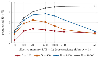
Proof. With $P_{t\mid t-1} = P_{t-1}/\lambda$ and unit noise variance, the Kalman gain is $P_{t\mid t-1}x_t/(1 + x_t^\top P_{t\mid t-1}x_t) = P_{t-1}x_t/(\lambda + x_t^\top P_{t-1}x_t) = k_t$ ; the state update is RLS’s; the filtered covariance $(I - k_tx_t^\top)P_{t\mid t-1} = (P_{t-1} - k_tx_t^\top P_{t-1})/\lambda$ is RLS’s $P_t$ . ∎

A forgetting factor is therefore an assumption about how fast the truth moves. Figure 12.1 measures the trade-off: short memories track regimes but estimate five coefficients from little data; long ones estimate well the coefficients of regimes that have ended. With regimes of 100 or 500 steps on average, the best memory is about 200 observations ( $\lambda = 0.995$ ), and it recovers 0.75% and 2.44% of R-squared out of a possible 4.9%; with regimes of 2 000 steps it is 500 observations (3.71%), and with regimes of 10 000 steps nothing should be forgotten ( $\lambda = 1$ , 5.21% of 5.29%). Online stochastic gradient descent with a fixed learning rate is a crude forgetting rule of its own (0.57%, 2.05%, 3.69% and 4.84%).

Prequential R-squared of recursive least squares (after 1 000 steps of warm-up) against its effective memory, for streams whose coefficients change every D steps on average. Data: ml_online.forgetting. — **Figure 12.1.** Prequential R-squared of recursive least squares (after 1 000 steps of warm-up) against its effective memory, for streams whose coefficients change every $D$ steps on average. Data: `ml_online.forgetting`.

12.3 Detecting drift

Definition 12.4 (Drift detector, Page–Hinkley test, adaptive windowing)

A drift detector watches a statistic of a model in production (its errors, its gains, a feature’s distribution) and raises an alarm when the statistic’s distribution appears to have changed. The Page–Hinkley test accumulates the deviations of the monitored value below its running mean, less a tolerance $\delta$ , and alarms when the sum rises more than $h$ above its running minimum (Page, 1954; Hinkley, 1971). Adaptive windowing (ADWIN) keeps a window of recent values and drops its older part whenever some split of the window into two sub-windows has means further apart than a Hoeffding-type bound at confidence $\delta$ (Bifet and Gavaldà, 2007).

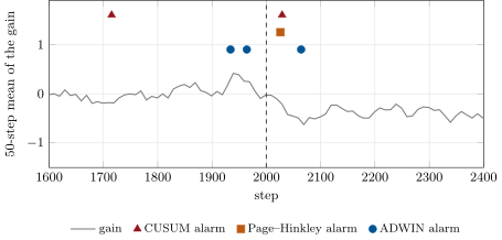
Book 7’s CUSUM test (chapter 13) is the third detector. All three watch the same statistic: the deployed model’s gain $g_t = \hat y_t\,y_t$ (its forecast times the outcome), standardised on the warm-up period, whose mean is positive while the model is right and falls when it is not. Their thresholds are set, on a long stream with no change, to one false alarm a year (one per 252 steps): $h = 9$ for CUSUM and Page–Hinkley (tolerance 0.1), $\delta = 0.0032$ for ADWIN. Then, on twenty streams whose coefficients reverse sign at step 2 000, the detectors raise their first true alarm after 20.8 steps on average for CUSUM (median 17), 27.4 for Page–Hinkley (median 18.5) and 42.5 for ADWIN (median 26.5); over the 1 000 steps before the reversal they raised 74, 78 and 91 false alarms across the twenty streams, close to the 79 their calibration implies (Figure 12.2).

One stream whose coefficients reverse at step 2 000 (dashed): the 50-step mean of the deployed model’s standardised gain, and each detector’s alarms from 300 steps before the reversal to its first alarm after it (markers at arbitrary heights, one row per detector). Data: ml_online. — **Figure 12.2.** One stream whose coefficients reverse at step 2 000 (dashed): the 50-step mean of the deployed model’s standardised gain, and each detector’s alarms from 300 steps before the reversal to its first alarm after it (markers at arbitrary heights, one row per detector). Data: `ml_online`.

12.4 Retraining schedules

Definition 12.5 (Retraining schedule)

A retraining schedule is the rule that decides when a model is refitted and on which data: on a calendar (every week, on a rolling window), on a detector’s alarm, continuously (an online estimator), or by a combination; it is part of the model and is validated with it.

schedule (least squares on the last 500 observations unless stated)	prequential $R^2$	refits
never (fitted on the first 1 000 steps)	$-7.81\%$	0
every 250 steps	2.62%	75
on a Page–Hinkley alarm (refit on the data since the alarm)	$-2.67\%$	2
recursive least squares, $\lambda = 0.998$	3.24%	every step
the truth	4.62%

Table 12.1. Four retraining schedules on a stream whose coefficients are redrawn every 2 000 steps on average (19 000 steps scored after a warm-up of 1 000). Data: ml_online.schedules.

Table 12.1 holds a lesson about detectors. The Page–Hinkley detector that caught a sign reversal within a median 18.5 steps refitted the model twice while the coefficients changed ten times: when coefficients are redrawn rather than reversed, the old model’s gains fall to zero rather than below it, a smaller change than it was tuned to fear, and it waits. The calendar schedule, dumb and regular, beats it; recursive least squares with the memory that suits the regimes beats both. A detector must be tuned to the change that matters, and a schedule that relies on one needs a calendar underneath it.

Method 12.6 (Choosing how a model adapts)

Estimate how fast the relation moves: fit the model on rolling windows of several lengths and compare their prequential scores, or equivalently scan the forgetting factor.
Score every schedule prequentially on history, including the costs of refitting (validation, deployment, turnover).
Calibrate detectors on periods without change to a false-alarm rate the desk can act on, and measure their delay on the changes that matter (a reversal, a fade to zero, a volatility shift).
Combine: a calendar refit as the floor, a detector to refit early, and an online estimator where the model is simple enough to update safely.

12.5 Tutorial: the half-life of a model

Goal. Scan the forgetting factor of recursive least squares against the regime length, calibrate three detectors to one false alarm a year and time them on a reversal, and compare retraining schedules. End state: Figures 12.1 and 12.2, Table 12.1.

Recursive least squares with forgetting (Proposition 12.3).

class RLS:
    """Minimises sum_s lam^(t-s) (y_s - x_s' b)^2; the effective memory is about 1 / (1 - lam) observations."""

    def __init__(self, p, lam=0.99, delta=100.0):
        self.b = np.zeros(p)
        self.P = delta * np.eye(p)
        self.lam = lam

    def predict(self, x):
        return float(x @ self.b)

    def update(self, x, y):
        Px = self.P @ x
        k = Px / (self.lam + x @ Px)
        self.b = self.b + k * (y - x @ self.b)
        P = (self.P - np.outer(k, Px)) / self.lam
        self.P = 0.5 * (P + P.T)                                         # keep P symmetric: rounding breaks it

Listing 12.1. Recursive least squares with a forgetting factor. code/firm/onlinelearn/firm_onlinelearn.py

The Page–Hinkley test.

class PageHinkley:
    """Page-Hinkley test for a fall in the mean: cumulate the deviations below the running mean (less a tolerance
    delta) and alarm when the cumulated sum rises lam above its running minimum."""

    def __init__(self, delta=0.0, lam=10.0):
        self.delta, self.lam = delta, lam
        self.reset()

    def reset(self):
        self.n, self.mean, self.m, self.mmin = 0, 0.0, 0.0, 0.0

    def update(self, v):
        self.n += 1
        self.mean += (v - self.mean) / self.n
        self.m += self.mean - v - self.delta
        self.mmin = min(self.mmin, self.m)
        if self.m - self.mmin > self.lam:
            self.reset()
            return True
        return False

Listing 12.2. The Page–Hinkley test for a fall in the mean. code/firm/onlinelearn/firm_onlinelearn.py

A windowed ADWIN.

class ADWIN:
    """Adaptive windowing (after Bifet and Gavalda): keep a window of recent values; drop its older part whenever some
    split into an older and a newer sub-window has means differing by more than a Hoeffding-type bound. Windowed
    O(window) version: splits are checked every `check` steps."""

    def __init__(self, delta=0.002, max_window=2000, check=5, min_side=30):
        self.delta, self.max_window, self.check, self.min_side = delta, max_window, check, min_side
        self.w: list[float] = []
        self.t = 0

    def update(self, v):
        self.w.append(v)
        if len(self.w) > self.max_window:
            self.w.pop(0)
        self.t += 1
        if self.t % self.check or len(self.w) < 2 * self.min_side:
            return False
        a = np.asarray(self.w)
        n = len(a)
        c = np.cumsum(a)
        i = np.arange(self.min_side, n - self.min_side)
        m0, m1 = c[i - 1] / i, (c[-1] - c[i - 1]) / (n - i)
        hm = 1.0 / (1.0 / i + 1.0 / (n - i))
        eps = np.sqrt(np.log(4 * n / self.delta) / (2 * hm)) * a.std()
        hit = np.abs(m0 - m1) > eps
        if hit.any():
            cut = int(i[np.flatnonzero(hit)[-1]])
            self.w = self.w[cut:]
            return True
        return False

Listing 12.3. Adaptive windowing, checked every few steps. code/firm/onlinelearn/firm_onlinelearn.py

Run ml_online.forgetting(D), thresholds(), delays(), schedules() and fig_online.py.

What to change next. Make the regimes fade their coefficients to zero instead of redrawing them and recalibrate the detectors for that change; combine the calendar with the detector.

12.6 Build: online learning and drift detection

Purpose. Models that adapt at a chosen speed, detectors with a known false-alarm rate, and schedules validated like the models they refit.

Interface. drift_stream(n, p, mean_regime, r2, seed, flip_at); RLS(p, lam, delta), OnlineSGD(p, lr), prequential(model, X, y); CUSUM(mu0, k, h), PageHinkley(delta, lam), ADWIN(delta, max_window, check, min_side), alarm_times, calibrate(make_for, thresholds, null_values, rate); retrain_schedule(X, y, policy, every, window, warm, make_detector, min_fit).

Rules. Predict before learning; detectors see only past and present values; thresholds come from calibration on no-change data, never from the period being judged.

Acceptance tests. code/firm/onlinelearn/tests/: RLS with $\lambda = 1$ equals batch least squares; its effective memory matches $1/(1-\lambda)$ on a planted change; each detector’s false-alarm rate on no-change data is within its calibration and it finds a planted mean shift; the calendar schedule refits at the right steps.

Stretch. Forgetting that adapts to the detector’s statistic (variable $\lambda$ ); detectors on feature distributions (chapter 27).

Sources and further reading

E. S. Page, “Continuous inspection schemes”, Biometrika 41(1/2), 1954.
A. Bifet and R. Gavaldà, “Learning from time-changing data with adaptive windowing”, SIAM International Conference on Data Mining, 2007.
J. Gama, I. Žliobaitė, A. Bifet, M. Pechenizkiy and others, “A survey on concept drift adaptation”, ACM Computing Surveys 46(4), 2014.
A. H. Sayed and T. Kailath, “A state-space approach to adaptive RLS filtering”, IEEE Signal Processing Magazine 11(3), 1994.
D. V. Hinkley, “Inference about the change-point from cumulative sum tests”, Biometrika 58(3), 1971.
G. Widmer and M. Kubat, “Learning in the presence of concept drift and hidden contexts”, Machine Learning 23, 1996.

12.7 Exercises

Exercise 12.1 ★

What are the effective memories of forgetting factors 0.99, 0.998 and 0.9995? What weight does an observation 500 steps old get with each, relative to the newest?

Solution

Solution of Exercise 12.1.

Memories $1/(1-\lambda)$ : 100, 500 and 2 000 observations. Relative weights $\lambda^{500}$ : $0.99^{500} = 0.0066$ , $0.998^{500} = 0.37$ , $0.9995^{500} = 0.78$ .

Exercise 12.2 ★

A detector raises one false alarm per 252 steps. How many false alarms should 20 streams of 1 000 steps raise? Compare with the chapter’s counts.

Solution

Solution of Exercise 12.2.

$20\times1\,000/252 = 79.4$ . The chapter’s 74, 78 and 91 are within the Poisson noise of that count ( $\pm9$ ), which is what a calibration on another no-change stream can promise.

Exercise 12.3 ★

A CUSUM with reference 0 and allowance $k = 0.1$ watches standardised gains whose mean falls from 0 to $-0.38$ at the reversal (the chapter’s streams). At what average rate does its statistic grow after the change, how many steps does it need from zero to pass $h = 9$ , and why is the measured median delay shorter?

Solution

Solution of Exercise 12.3.

The statistic adds $\mu_0 - v - k$ each step, on average $0 + 0.38 - 0.1 = 0.28$ ; from zero it needs $9/0.28\approx32$ steps. The measured median is 17 because the statistic does not start at zero: under no change a reflected walk with drift $-0.1$ and unit variance sits on average at about $1/(2\times0.1) = 5$ , so at the change it is typically a few units up already, and noise makes the first passage earlier still.

Exercise 12.4 ★★

Why does the best memory grow with the regime length, and why is it not proportional to it?

Solution

Solution of Exercise 12.4.

The error of a forgetting estimator has two parts: estimation noise, which falls as the memory $M$ grows (about $p/M$ in R-squared units), and staleness, which grows with the share of the memory spent in past regimes (about $M/D$ times the signal). Minimising $p/M + cM/D$ gives $M\propto\sqrt{pD/c}$ : the best memory grows like the square root of the regime length, not in proportion to it. The chapter’s optimum, 200 observations at $D = 100$ and 500 at $D = 2\,000$ , fits that slow growth; at $D = 10\,000$ the stream holds only two regimes and forgetting nothing wins.

Exercise 12.5 ★★

Why did the Page–Hinkley schedule refit only twice, and what would you change?

Solution

Solution of Exercise 12.5.

It was calibrated and timed on sign reversals, where the gains fall to about $-0.38$ standard deviations; when the coefficients are redrawn at random the old model’s gains fall only to about zero, a change of half the size, and a threshold of 9 with a tolerance of 0.1 needs a long run of them. Recalibrate the tolerance for the change that matters (fading to zero), watch a statistic that responds to it (the rolling correlation of forecast and outcome), and keep a calendar refit as a floor under the detector.

Exercise 12.6 ★★

Find the flaw. “We chose the detector’s threshold so that it caught last year’s two regime changes within a week, and it would have.”

Solution

Solution of Exercise 12.6.

The threshold was tuned on the two changes it is then judged on: its delay is measured in-sample and its false-alarm rate is not measured at all. Two events cannot calibrate anything. Set the threshold on no-change data to a chosen false-alarm rate, then measure the delay on changes the threshold never saw (planted ones, or later history).

Exercise 12.7 ★★★

Coding. Run ml_online.schedules with regimes of 500 steps on average (schedules(D=500)). Report the four schedules and explain what changed.

Solution

Solution of Exercise 12.7.

With regimes of 500 steps on average: never refitted $-3.68\%$ ; every 250 steps $-0.60\%$ (75 refits); on a Page–Hinkley alarm $-8.24\%$ (45 refits); recursive least squares with $\lambda = 0.995$ 2.24%; the truth 5.35%. The calendar schedule’s 500-observation window now spans a regime change most of the time, so its fits are stale; the detector alarms far more often and each time refits on the 100 observations since the alarm, five coefficients from a sample too small for a signal worth 5% of the variance, and those noisy fits lose more than a stale one. Only the estimator whose memory suits the regimes, about 200 observations, stays positive.

Exercise 12.8 ★★★

Show that RLS with $\lambda = 1$ and $P_0 = \delta I$ gives the ridge estimator with penalty $1/\delta$ , and hence ordinary least squares as $\delta\to\infty$ .

Solution

Solution of Exercise 12.8.

With $\lambda = 1$ the update of $P$ is the Sherman–Morrison formula for $P_t^{-1} = P_{t-1}^{-1} + x_tx_t^\top$ , so $P_t^{-1} = I/\delta + \sum_{s\le t}x_sx_s^\top$ . By induction, $P_t^{-1}\hat\beta_t = \sum_{s\le t}x_sy_s$ : it holds at $t = 0$ with $\hat\beta_0 = 0$ , and $P_t^{-1}\hat\beta_t = P_t^{-1}\hat\beta_{t-1} + P_t^{-1}k_t(y_t - x_t^\top\hat\beta_{t-1})$ with $P_t^{-1}k_t = x_t$ gives $P_{t-1}^{-1}\hat\beta_{t-1} + x_ty_t$ . Hence $\hat\beta_t = (X^\top X + I/\delta)^{-1}X^\top y$ , the ridge estimator with penalty $1/\delta$ , which tends to ordinary least squares as $\delta\to\infty$ .

12.8 Problem: The Half-Life of a Model

Problem 12.1

Weekend problem — how fast to forget

The chapter’s stream: five features, a signal worth 5% of the variance, coefficients redrawn every $D$ steps on average.

Part I — Forgetting.

What is the truth’s R-squared, and why is no model close to it for short regimes?
Which forgetting factor is best for $D = 100$ , 500, 2 000 and 10 000, and what does it score?
What does online SGD score, and why does it behave like forgetting?
What does Proposition 12.3 say a forgetting factor assumes?

Part II — Detectors.

What statistic do the detectors watch, and why the gain rather than the squared error?
What thresholds give one false alarm a year?
What are their mean and median delays after a reversal?
How many false alarms did they raise before the reversal, and is that too many?

Part III — Schedules.

What do the four schedules score with regimes of 2 000 steps?
Why does the never-refitted model score below zero?
Why did the detector-driven schedule fail?
Why does recursive least squares win?

Part IV — The verdict.

State the named result: the forgetting factor that minimises the out-of-sample loss as a function of the regime length, and each detector’s delay at one false alarm a year.
What schedule would you run for a short-horizon model on a changing venue?
How would you estimate $D$ on real data?
What does a false alarm cost, and what does a missed change cost?
How does this chapter connect to Book 7’s signal half-life?
What should a monitoring system log for each alarm?
How would covariate shift show up in these statistics?
In one sentence: how fast should a model forget?

Solution

Solution of Problem 12.1.

Part I.

4.9% to 5.4% depending on the stream. With regimes of 100 steps the model must estimate five coefficients from about a hundred observations before they change; its estimation noise is as large as the signal.
$\lambda = 0.995$ (memory 200) for $D = 100$ and 500, scoring 0.75% and 2.44%; $\lambda = 0.998$ (500) for $D = 2\,000$ , 3.71%; $\lambda = 1$ for $D = 10\,000$ , 5.21% against the truth’s 5.29%.
0.57%, 2.05%, 3.69% and 4.84%. A fixed learning rate weights old observations geometrically, like a forgetting factor, but along one gradient direction at a time; it is a cheaper and noisier version of RLS.
That the true coefficients follow a random walk, with a variance per step set by $\lambda$ : choosing $\lambda$ is choosing how fast you believe the truth moves.

Part II.

The gain $\hat y_ty_t$ , standardised on the warm-up. It is what the desk earns from the model, and its mean changes sign when the relation reverses; the squared error is dominated by the noise, which does not change.
$h = 9$ for CUSUM and Page–Hinkley (allowance and tolerance 0.1), $\delta = 0.0032$ for ADWIN.
CUSUM 20.8 (median 17), Page–Hinkley 27.4 (18.5), ADWIN 42.5 (26.5) steps.
74, 78 and 91 over 20 000 steps, against 79 expected: as calibrated. Whether one a year is too many is the desk’s cost question (Part IV).

Part III.

Never $-7.81\%$ ; every 250 steps 2.62%; on a Page–Hinkley alarm $-2.67\%$ (two refits); RLS with $\lambda = 0.998$ 3.24%; the truth 4.62%.
Its coefficients belong to the first regime; in the other regimes they are unrelated or opposite to the truth, and a forecast that is wrong in direction scores below the zero forecast.
It was tuned to reversals and the stream redraws; see Exercise 12.5.
It refits every step with the memory that suits the regimes, with no threshold to cross and no sample thrown away.

Part IV.

The half-life of a model. The forgetting factor that minimises the prequential loss grows with the regime length: $\lambda = 0.995$ at $D = 100$ and 500, 0.998 at 2 000, 1 at 10 000. At one false alarm per 252 steps, the median delay to a sign reversal is 17 steps for CUSUM, 18.5 for Page–Hinkley and 26.5 for ADWIN.
An online estimator where the model is linear or has a linear last layer, with the memory chosen on history; a calendar refit of the rest; a detector on the gains to trigger an early refit and a human review.
Scan the forgetting factor or the rolling window on history and read the regime length off the optimum (Exercise 12.4); or count the breaks Book 7’s tests find.
A false alarm costs a refit (compute, validation, a new model’s turnover) and trust; a missed change costs the losses of a wrong model until the next refit, which for a reversed signal is the whole position’s expected loss.
Book 7 measured a signal’s decay after the fact; the forgetting factor turns that half-life into the memory of the estimator that trades the signal.
The time, the detector and its threshold, the statistic’s path, the model version, and what was done: refit, override, or dismissed, with a reason.
As a change in the features’ distribution with the gains unchanged; detectors on the features (chapter 27) see it, detectors on the gains do not until it hurts.
As fast as the truth moves and no faster, which you measure on history and check on the gains.

12.9 Interview questions

Interview question 12.1 ★ mle, researcher

What is the difference between concept drift and covariate shift? Give a market example of each.

Solution

Solution of Interview question 12.1.

Concept drift changes $\P(y\mid x)$ : a signal crowds out, or a fee change reverses the sign of an order-flow feature’s effect. Covariate shift changes $\P(x)$ only: a volatility regime moves features into ranges the model rarely saw.

What the interviewer is looking for: the two distributions and a correct example of each.

Interview question 12.2 ★★ researcher

Derive recursive least squares with a forgetting factor, and say what the forgetting factor means.

Solution

Solution of Interview question 12.2.

Minimise $\sum_s\lambda^{t-s}(y_s - x_s^\top b)^2$ ; the normal equations $R_tb = r_t$ with $R_t = \lambda R_{t-1} + x_tx_t^\top$ and $r_t = \lambda r_{t-1} + x_ty_t$ ; Sherman–Morrison on $P_t = R_t^{-1}$ gives the gain, the coefficient update and the covariance update of Definition 12.2. $\lambda$ sets the memory, about $1/(1-\lambda)$ observations.

What the interviewer is looking for: the weighted objective, the rank-one update, and the memory interpretation.

Interview question 12.3 ★★ mle

How do you set the threshold of a drift detector, and how do you know it works?

Solution

Solution of Interview question 12.3.

On data with no change, pick the threshold that gives the false-alarm rate the desk can act on; then plant the changes that matter and measure the delay; report both. Check on held-out history that the rate holds.

What the interviewer is looking for: calibration on no-change data, a delay measured on unseen changes, and the trade-off between them.

Interview question 12.4 ★★ researcher, trader

Your model is retrained monthly. How would you decide whether to retrain weekly, daily, or continuously?

Solution

Solution of Interview question 12.4.

Score each schedule prequentially on history, costs of refitting included; estimate how fast the relation moves (the forgetting-factor or window scan); weigh the gain against the operational risk of more frequent deployments; keep the calendar as a floor and add a detector.

What the interviewer is looking for: a prequential comparison, costs, and a drift estimate.

Interview question 12.5 ★★ mle

Explain the Page–Hinkley test and one weakness of it.

Solution

Solution of Interview question 12.5.

It accumulates the deviations of the value below its running mean, less a tolerance, and alarms when the sum rises a threshold above its running minimum. Weaknesses: the running mean includes all history since the last reset, so after a long calm period it reacts slowly; it detects one direction and one size of change well, the one its tolerance and threshold were tuned to.

What the interviewer is looking for: the statistic and a real weakness (memory of the running mean, or tuning to one change).

Interview question 12.6 ★★★ researcher

Show that exponential forgetting is a Kalman filter for a random-walk coefficient, and what that implies for choosing $\lambda$ .

Solution

Solution of Interview question 12.6.

See Proposition 12.3: inflating the state covariance by $1/\lambda$ in the prediction step reproduces RLS. So $\lambda$ encodes how fast the coefficients move relative to the noise; choose it by scoring on history, or estimate the state noise by maximum likelihood and read off the implied $\lambda$ .

What the interviewer is looking for: the prediction step matched to the forgetting and the implication for choosing $\lambda$ .

Terms defined in this chapter

See all 2333 terms in the glossary