18Reinforcement Learning for Execution and Market Making

Execution and market making both have optimal policies in closed form in their textbook models: the Almgren–Chriss schedule (Book 10, chapter 14) and the inventory-aware quotes of Book 11 (chapter 3). The reason to learn a policy instead is everything the textbook model leaves out; the risk, as chapter 17 showed, is that a learned policy exploits what its training world gets wrong. This chapter measures both on problems whose optimum is known. A deep Q-network learns the Almgren–Chriss schedule to within 0.4 basis points; moved to a market whose impact is three times higher, it loses 9.1 basis points to that market’s optimum, four times what the textbook schedule of the wrong model loses. Trained on randomised impact and allowed to see the impact of its own fills, it loses 0.9 there and 0.6 at home. A tabular learner for market making, given 1.6 million steps, still falls short of the closed form and of a constant quote.

18.1 State, action and reward design

Definition 18.1 (Reward shaping, action masking)

Reward shaping changes the rewards an agent learns from without changing the policy that is optimal, for instance by removing a term whose expectation is known to be zero, or by adding a potential difference, to make learning faster or more stable. Action masking removes the actions that are not allowed in a state (selling more than is held, quoting a side that would breach an inventory limit) from the agent’s choice and from the maximum in its learning target.

Design decides most of what an agent can learn. The execution agent sells one unit over ten steps in lots of a twentieth; its state is the time, the holdings and one number described below; its action is the number of lots to sell, with every sale above the holdings masked and the whole remainder forced at the last step. Its reward is the Almgren–Chriss objective split by step: minus the temporary-impact cost $\eta u^2/\tau$ of the sale, minus the risk charge $\lambda\sigma^2\tau x^2$ on what is still held, with $\eta = 0.001$, $\sigma = 0.02$ and $\lambda = 10$ (in basis points, TWAP costs 21.4 and the optimum 18.85). The realised P&L of the holdings over the step, $\sigma\sqrt\tau Z x$, has expectation zero; leaving it out is reward shaping. Leaving it in is not harmless: with that noise in its reward, the same network after the same 1 500 episodes learned to sell the same amount every step, TWAP exactly, 2.55 basis points from the optimum.

18.2 Deep Q-networks and their stabilisers

Definition 18.2 (Deep Q-network, experience replay, target network)

A deep Q-network (DQN) is Q-learning (chapter 17) with the action-value function represented by a neural network, trained by stochastic gradient steps on the temporal-difference error (Mnih and co-authors, 2015). Two stabilisers make it work: experience replay stores past transitions and trains on random batches of them, breaking the correlation of consecutive steps; a target network is a copy of the network, updated only every few hundred steps, used to compute the learning targets so that they do not move with every update.

The chapter’s DQN (Listing 18.1) is a two-layer network of 64 units with 21 outputs, a replay memory of 20 000 transitions, a target network copied every 200 updates and exploration decaying from 1 to 0.05 over the first half of training. After 1 500 episodes its greedy schedule costs 19.29 basis points, 0.44 above the continuous Almgren–Chriss optimum; 0.20 of that gap is the lot grid, whose own optimum costs 19.05. Maximisation over noisy estimates biases Q-learning upwards; double Q-learning, which chooses the action with one network and values it with the other (van Hasselt, Guez and Silver, 2016), is the usual remedy and the design Ning and co-authors (2021) used for execution.

18.3 Learning to execute

Definition 18.3 (Domain randomisation)

Domain randomisation trains a policy on many versions of a simulator whose uncertain parameters are drawn at random for each episode, so that the policy works across them instead of exploiting one (Tobin and co-authors, 2017).

The textbook’s weakness is its parameters: impact is estimated with error and changes with the market. Three worlds test the agents: the model’s ($\eta = 0.001$), a market with three times the impact, and one with a third of it; each has its own Almgren–Chriss optimum, and every schedule is scored exactly against it (Figure 18.1). The third state variable is the impact the agent has observed in its own fills so far, as the logarithm of its ratio to the model’s value (zero before the first sale): a real execution algorithm measures its impact as it trades.

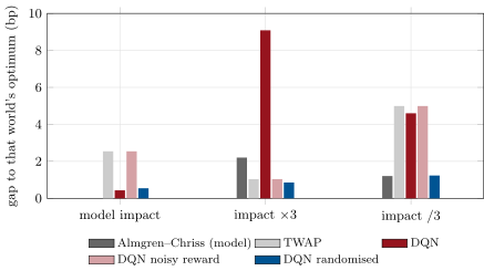
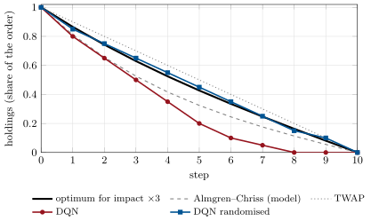
The model-trained DQN is the chapter’s warning. In its own world it is 0.44 from the optimum; where impact is three times higher it is 9.09 away, and where impact is lower 4.60: it has never seen its third input take those values, and a network off its training distribution does something arbitrary. The closed form built on the same wrong impact loses 2.20 and 1.21: a formula degrades smoothly where a network need not. The randomised DQN, trained for 3 000 episodes with the impact drawn anew each episode, learned to read its fills: it sells a little more slowly than the model’s optimum at first and then follows the impact it observes, and its gaps are 0.55, 0.86 and 1.24: the best of all in the high-impact world, and within 0.03 of the best (the closed form, by luck of the direction of its error) in the low-impact one. Figure 18.2 shows the schedules in the high-impact world.

18.4 Learning to make markets

Market making in the model of Book 11 (chapter 3) has an exact solution: a mid-price that diffuses, fills at depth $\delta$ with intensity $Ae^{-k\delta}$, a running penalty $\phi q^2$ on inventory and a terminal penalty $\alpha q^2$, here with $A = 140$, $k = 1.5$, $\sigma = 2$, $\phi = 0.02$, $\alpha = 0.01$ and inventory within $\pm10$. The optimal depths at the start are 0.68 on both sides when flat and 0.57 and 0.79 when five units long (tighter on the side that reduces inventory). The learner is tabular Q-learning (Listing 18.2) over 20 time buckets and the 21 inventories, choosing each side’s depth among six values, with the zero-mean inventory P&L shaped out of its reward and inventory-breaching sides masked. Table 18.1 scores every policy with the firm’s market-making simulator on 5 000 common paths.

policy	objective	(s.e.)	P&L s.d.	$|q_T|$	fills
exact optimum (Book 11)	67.95	0.12	8.53	2.67	101.8
Avellaneda–Stoikov, $\gamma = 0.1$	64.73	0.09	6.50	2.26	97.0
constant depth $1/k$	66.67	0.17	11.61	5.03	101.0
Q-learning, 2 000 episodes	62.34	0.12	8.31	4.40	91.7
Q-learning, 8 000 episodes	62.84	0.12	8.53	4.38	93.1

The learner improves slowly and stays below the constant quote: 1.6 million steps of experience are not enough to rank six depths whose expected values differ by less than the noise of a fill. The spread earned per step is a small signal under a large noise, which is the market maker’s problem in general. Closed forms or parametric policies fitted by policy search in a simulator (a depth that is a line in inventory has two parameters, where the table has 420 states and 36 actions) are what work at this scale; learning earns its place on the parts the model leaves out, such as queue position, adverse selection and several venues, where no closed form exists.

18.5 What works in the published evidence

The evidence is thinner than the attention. Nevmyvaka, Feng and Kearns (2006) applied reinforcement learning to execution on a year and a half of millisecond limit-order data from NASDAQ, with a state space factorised to keep learning tractable; Ning and co-authors (2021) trained a double deep Q-network with experience replay on order-book features for nine stocks and found it beat the standard benchmark on most of them; Spooner and co-authors (2018) built a high-fidelity limit-order-book simulator and a temporal-difference market maker with a custom reward that controls inventory risk, which beat simple benchmarks and an online-learning approach in that simulator. Hambly, Xu and Yang (2023) survey the field. The common thread is the simulator: results are reported in a simulator, often the authors’ own, and the transfer to live trading is rarely documented in public. A desk should read them as evidence that the methods work where the simulator is right, and build its own evidence with the tests of chapter 17 and this chapter: exact benchmarks, several worlds, off-policy evaluation on its own logs.

Method 18.4 (Deploying a learned execution or quoting policy)

1. Benchmark against the closed form of the textbook model in that model; a learner that cannot match it there is not ready.
2. Shape rewards to remove known zero-mean noise, mask forbidden actions, and give the state the signals a trader would use (fills, observed impact, queue position).
3. Train on randomised simulators whose parameters span their estimation error, and evaluate in held-out parameter settings, never only in the training one.
4. Bound the policy (participation limits, inventory limits, a fallback to the closed form) and compare live against the incumbent by off-policy evaluation and small controlled trials.

18.6 Tutorial: beating a closed form

18.7 Build: trading environments and learners

18.8 Exercises

Exercise 18.1 ★

Compute TWAP’s objective in the model world: ten sales of 0.1 with $\eta = 0.001$, $\tau = 0.1$, and the risk charge with $\sigma = 0.02$, $\lambda = 10$. Give it in basis points.

Solution

Solution of Exercise 18.1.

Impact: $10\times0.001\times0.1^2/0.1 = 0.001$. Risk: $10\times0.02^2\times0.1\times(0.9^2 + 0.8^2 + \dots + 0.1^2) = 0.0004\times2.85 = 0.00114$. Total $0.00214$, or 21.4 basis points.

Exercise 18.2 ★

At what depth does $\delta Ae^{-k\delta}$, the expected spread earned per unit time on one side, peak? Compare with the exact optimum’s flat depth.

Solution

Solution of Exercise 18.2.

$\frac{d}{d\delta}\delta e^{-k\delta} = (1 - k\delta)e^{-k\delta} = 0$ at $\delta = 1/k = 0.67$. The exact optimum’s flat depth at the start is 0.68: the inventory penalties widen it slightly, since each fill adds inventory risk.

Exercise 18.3 ★

Why must the mask also enter the target $\max_{u'}Q(x', u')$, not only the choice of action?

Solution

Solution of Exercise 18.3.

The target values the next state by its best action; if forbidden actions enter the maximum, the agent learns values it can never collect (selling more than it holds, skipping the forced final sale), and those inflated values propagate back to every earlier state.

Exercise 18.4 ★★

Show that removing $\sigma\sqrt\tau Zx$ from each step’s reward leaves the optimal policy unchanged. Why did the noisy agent end at TWAP?

Solution

Solution of Exercise 18.4.

$Z$ is independent of everything the agent knows and chooses, so $\E[\sigma\sqrt\tau Zx_k\mid\text{history}] = 0$ for any policy: every policy’s expected return is unchanged, hence the optimal policy is. The term’s standard deviation, about $63x$ basis points per step, dwarfs the differences between schedules (a few basis points in all), so with the noise the network’s value estimates were dominated by it after 1 500 episodes and its greedy choice was the flat schedule; with more episodes it would improve, slowly.

Exercise 18.5 ★★

Why did the model-trained DQN do worse than the wrong closed form in the high-impact world?

Solution

Solution of Exercise 18.5.

Its third input, the observed impact, was always zero in training (the impact never varied), so the network’s response to other values was never constrained; at $\log3$ it produced an arbitrary schedule. The closed form of the wrong model is at least a sensible schedule for a nearby world, and its error grows smoothly with the parameter error.

Exercise 18.6 ★★

Find the flaw. “We trained the market maker with domain randomisation over volatility and it was profitable in every one of 10 000 randomised simulator runs, so it is robust.”

Solution

Solution of Exercise 18.6.

Robustness to volatility says nothing about what was not randomised (fill model, adverse selection, latency, other market makers) and nothing about the simulator’s structure; 10 000 runs of one simulator are one piece of evidence. Test in worlds that differ in the unrandomised assumptions, and on real logs.

Exercise 18.7 ★★★

Coding. Replace the market maker’s table by the policy $\delta_{b,a} = c\pm dq$ and choose $(c, d)$ on a grid by the simulator’s mean objective on 2 000 paths. How close do you get to the exact optimum?

Solution

Solution of Exercise 18.7.

The grid search chooses $c = 0.70$ and $d = 0.03$ on 2 000 paths; on the chapter’s 5 000 common paths the policy scores 67.82, against 67.95 for the exact optimum and 62.84 for the table after 8 000 episodes. Two well-chosen parameters recover almost everything, which is the argument for structure over tables.

Exercise 18.8 ★★★

Derive the discrete Almgren–Chriss schedule for the chapter’s objective by writing the first-order conditions in the holdings $x_1,\dots,x_{n-1}$.

Solution

Solution of Exercise 18.8.

Minimise $\sum_{k=1}^n\eta(x_{k-1} - x_k)^2/\tau + \lambda\sigma^2\tau\sum_{k=1}^{n-1}x_k^2$ with $x_0 = X$, $x_n = 0$. The derivative in $x_k$ gives $-2\eta(x_{k-1} - x_k)/\tau + 2\eta(x_k - x_{k+1})/\tau + 2\lambda\sigma^2\tau x_k = 0$, that is $x_{k-1} - 2x_k + x_{k+1} = (\lambda\sigma^2\tau^2/\eta)x_k$. The solutions are combinations of $e^{\pm\tilde\kappa t_k}$ with $2(\cosh\tilde\kappa\tau - 1) = \lambda\sigma^2\tau^2/\eta$; the boundary conditions give $x_k = X\sinh(\tilde\kappa(T - t_k))/\sinh(\tilde\kappa T)$, the schedule of firm.acexec.discrete.

18.9 Problem: Beating a Closed Form

Problem 18.1

Weekend problem — when to learn a policy

The chapter’s liquidation and market-making problems.

Part I — Design.

1. What are the execution agent’s state, actions and reward?
2. Why is the P&L noise removed from the reward, and what happened when it was not?
3. What does action masking prevent?
4. Why give the agent the impact it has observed?

Part II — Execution.

5. What do TWAP, the lot-grid optimum and the DQN cost in the model world?
6. What are the gaps of each schedule in the three worlds?
7. Why does the randomised agent lose a little at home?
8. What would change with a price that trends during the order?

Part III — Market making.

9. What are the exact optimum’s depths at the start?
10. How do the five policies score?
11. Why does the tabular learner stay below a constant quote?
12. What would you learn, and what would you keep in closed form?

Part IV — The verdict.

13. State the named result: the learned policy’s shortfall against the Almgren–Chriss optimum in the model world and in the mis-specified worlds, with and without domain randomisation.
14. What does the published evidence show, and what does it not?
15. How would you deploy the randomised execution agent?
16. What is the fallback if the agent’s observed impact leaves its training range?
17. Why does a table not scale to a real order book?
18. Which stabiliser matters most in the DQN here, and how would you check?
19. What should the comparison with the incumbent algorithm look like?
20. In one sentence: when is a learned policy worth more than a closed form?

Solution

Solution of Problem 18.1.

Part I.

1. State: time, holdings, observed impact; actions: lots to sell (masked); reward: minus impact cost minus risk charge.
2. Its expectation is zero, so it only adds variance; with it, the DQN learned TWAP (2.55 basis points from the optimum).
3. Selling more than is held, and anything but the whole remainder at the last step, in both the choice and the target.
4. It is what a trader would use to adapt, and it lets a policy trained on many impacts act on the one it meets.

Part II.

1. TWAP 21.40, lot-grid optimum 19.05, DQN 19.29 basis points (continuous optimum 18.85).
2. Model world, impact $\times3$, impact $/3$: closed form of the model 0, 2.20, 1.21; TWAP 2.55, 1.04, 4.99; DQN 0.44, 9.09, 4.60; DQN with noisy reward 2.55, 1.04, 4.99; randomised DQN 0.55, 0.86, 1.24.
3. Before its first sale it does not know the impact, so its first step hedges across the range it was trained on.
4. The objective would gain a drift term; a signal in the state would let the agent learn to trade with it, and to overfit it.

Part III.

1. 0.68 on both sides when flat; 0.57 on the ask and 0.79 on the bid when five units long.
2. Exact optimum 67.95; Avellaneda–Stoikov 64.73; constant $1/k$ 66.67; Q-learning 62.34 after 2 000 episodes and 62.84 after 8 000.
3. The expected values of neighbouring depths differ by less than the noise of the fills it sees; each of 15 120 table entries is estimated from few, noisy samples.
4. Keep the structure (depths as functions of inventory and time, from the closed form or a parametric family) and learn what the model omits: adverse selection, queue position, the fill model.

Part IV.

1. Beating a closed form. The DQN trained on the model’s impact is 0.44 basis points from the Almgren–Chriss optimum at home and 9.09 and 4.60 in worlds with three times and a third of the impact; trained with domain randomisation and the observed impact in its state, 0.55, 0.86 and 1.24.
2. That the methods work in simulators, often the authors’ own, and in some backtests on real data; not how the policies did live, which is rarely public.
3. Inside participation limits, with the closed form as fallback, compared with the incumbent by off-policy evaluation and a small randomised trial, and with its observed-impact input monitored.
4. Revert to the closed form with the impact re-estimated; do not let the network act outside the range it was trained on.
5. The state (queue positions, book levels, prices) is continuous and large; tables have no generalisation.
6. The target network and masking; ablate each and compare learning curves across seeds.
7. Paired comparison on the same orders or alternating orders, costs measured against arrival price, with enough orders for the difference’s standard error to be below the effect.
8. When the problem has parts no closed form captures and a simulator or logs good enough to learn them.

18.10 Interview questions

Interview question 18.1 ★ mle

What are experience replay and target networks for?

Solution

Solution of Interview question 18.1.

Replay breaks the correlation of consecutive samples and reuses data; the target network keeps the regression target fixed for a while, so the network does not chase its own moving estimates.

What the interviewer is looking for: both mechanisms and the instability each addresses.

Interview question 18.2 ★★ researcher, trader

How would you frame optimal execution as a reinforcement-learning problem? What goes in the state?

Solution

Solution of Interview question 18.2.

Episodes are parent orders; state: time left, quantity left, spread, depth, recent volatility, queue position, observed impact; actions: child-order sizes and types; reward: minus implementation shortfall increments with a risk term; benchmarks: Almgren–Chriss and the desk’s algorithm.

What the interviewer is looking for: state, action, reward and a benchmark.

Interview question 18.3 ★★ researcher

What is reward shaping, and how can it go wrong?

Solution

Solution of Interview question 18.3.

Changing rewards to ease learning without changing the optimal policy (removing zero-mean noise, potential-based terms). It goes wrong when the change alters incentives: a bonus for fills that teaches the agent to cross the spread, an inventory penalty that is not the risk the desk cares about.

What the interviewer is looking for: the invariance condition and an example of a harmful shaping.

Interview question 18.4 ★★ mle

Your DQN’s Q-values keep growing during training. What is happening and what do you do?

Solution

Solution of Interview question 18.4.

Overestimation from maximising over noisy estimates, possibly divergence from bootstrapping with function approximation. Use double Q-learning, a slower target update, smaller learning rate, reward scaling or clipping, and check that masked actions are excluded from the target.

What the interviewer is looking for: maximisation bias and concrete remedies.

Interview question 18.5 ★★ researcher, trader

Would you use reinforcement learning for market making? Where would it help and where not?

Solution

Solution of Interview question 18.5.

Where the closed forms omit things that matter (adverse selection, queue dynamics, several venues) and a good simulator or logs exist, with structure kept in the policy. Not for learning what a closed form already gives, where the signal per decision is too small to learn from fills.

What the interviewer is looking for: structure first, learning for the omitted parts, and the signal-to-noise problem.

Interview question 18.6 ★★★ researcher

What is domain randomisation, and why can it help and hurt a trading policy?

Solution

Solution of Interview question 18.6.

Training over many simulator parameter draws so that the policy works across them. It helps when the true parameters are in the range and the state lets the policy infer them; it hurts when the range is wrong or too wide (the policy hedges and loses at home) or when the unrandomised structure is what is wrong.

What the interviewer is looking for: what it buys, the observability condition, and its costs.